Module objectives
By the end of this module, you should be able to
- Define and explain the terms associated with eigenvectors.
- Describe and implement the power method.
- Understand how the power method is used in the page-rank algorithm.
- Describe the QR algorithm.
11.0
Some examples and definitions
As we've seen, there are two interpretations of \({\bf Ax}={\bf b}\):
- The numbers in \({\bf x}\) are the scalars in the linear
combination of the columns of \({\bf A}\), which results in vector
\({\bf b}\).
- Matrix \({\bf A}\) "acts" on vector \({\bf x}\) to
produce vector \({\bf b}\).
We will focus on the second interpretation.
Let's start with some examples of a matrix transforming a vector.
In-Class Exercise 1:
Download MatrixVectorExample.java
and examine the code. Notice that a matrix \({\bf A}\) multiplies
the vector \({\bf u}\) to produce vector \({\bf v}\), plotting
both vectors. Observe what happens when
- \({\bf u}=(0,1)\)
- \({\bf u}=(1,2)\)
- \({\bf u}=(1,0)\)
- \({\bf u}=(1,0)\) and \({\bf A}[0][0] = -5\).
We observe that the same matrix can sometimes:
- Change a vector's direction and length.
- Have no effect on both direction and length.
- Change only the length, keeping the direction.
- Flip the direction (while perhaps also changing the length).
We'll now explore the idea of repeatedly applying a matrix
iteratively:
- That is,
    u = some initial vector
    draw (u)
    for i=0 ...
       u = A u
       draw (u)
    endfor
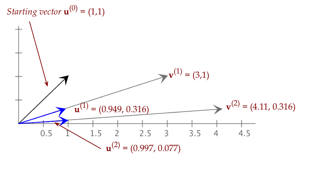
- Mathematically, we would describe this as the
iteration \({\bf u}^{(k)} = {\bf A}{\bf u}^{(k-1)}\):
- Let \({\bf u}^{(0)}\) be an initial vector.
- The superscript denotes the iteration number.
- After the first iteration, we get
\({\bf u}^{(1)} = {\bf A}{\bf u}^{(0)}\)
- After the second iteration, we get
\({\bf u}^{(2)} = {\bf A}{\bf u}^{(1)}\)
- And so on.
In-Class Exercise 2:
Download MatrixVectorExample2.java
and examine the code to verify that an initial vector
is iteratively multiplied by a matrix.
(You will also need
DrawTool.java).
Observe what happens when we change the starting vector to:
- \({\bf u}=(1,1)\)
- \({\bf u}=(0,1)\)
- \({\bf u}=(0.1,1)\)
- \({\bf u}=(1,2)\)
- \({\bf u}=(1.1,2)\)
- \({\bf u}=(1.01,2)\)
Observe that:
- In all but one case, the iteration converges to the
same positive or negative direction.
\(\rhd\)
In case, to the (1,0) direction.
- The only case when it's different is when
\({\bf u}^{(0)} = (1,2)\).
Note: we will consider "same direction" to mean either positive
or negative (flipped).
Eigenvalues and eigenvectors:
- Definition:
A vector \({\bf x}\) is called an eigenvector of
matrix \({\bf A}\) if
$${\bf Ax}=\lambda{\bf x}$$
for some number \(\lambda\).
- Definition: The scalar \(\lambda\) is
called the eigenvalue associated with the eigenvector
\({\bf x}\).
- In other words, when \({\bf A}\) multiplies \({\bf x}\),
we get a result vector \(\lambda{\bf x}\) in the same
direction.
- Example:
$$
\mat{5 & -2\\
0 & 1}
\vectwo{1}{0}
\eql
\vectwo{5}{0}
\eql
5
\vectwo{1}{0}
$$
Here \({\bf x}=(1,0)\) is an eigenvector with eigenvalue
\(\lambda=5\).
In-Class Exercise 3:
Show that \((1,2)\) is an eigenvector for the above matrix.
What is the associated eigenvalue?
In-Class Exercise 4:
Suppose \({\bf Ax}=\lambda{\bf x}\). Let \({\bf y}=-2{\bf x}\).
Show that \({\bf y}\) is an eigenvector of \({\bf A}\). What
is the associated eigenvalue?
- Thus, an eigenvector is not unique: given an eigenvector
\({\bf x}\), any other vector \(\alpha{\bf x}\) for any \(\alpha\)
is also an eigenvector.
- Note: the matrix \({\bf A}\) in \({\bf Ax}=\lambda{\bf x}\)
needs to be square:
- Consider \({\bf A}_{m\times n} {\bf x}_{n\times 1}\).
- This produces a vector of dimension \(m\times 1\).
- The only way \({\bf Ax}=\lambda{\bf x}\) is if \(m=n\).
In-Class Exercise 5:
Show by hand that \({\bf x}_1=(\frac{1}{\sqrt{2}},\frac{1}{\sqrt{2}})\)
and \({\bf x}_2=(\frac{1}{\sqrt{2}},-\frac{1}{\sqrt{2}})\)
are eigenvectors of \({\bf A}=\mat{2 & 1\\1 & 2}\).
What are the associated eigenvalues?
In-Class Exercise 6:
Download MatrixVectorExample3D.java,
compile and execute to see an example of repeated iteration
(\({\bf u} \leftarrow {\bf Au}\)) in 3D.
11.1
The power method
Iterative application of \({\bf A}\):
In-Class Exercise 9:
Download PowerMethodExample.java,
compile and execute.
For illustration, the code also computes
\({\bf A}^k {\bf u}^{(0)}\).
Is the resulting vector the same eigenvector as computed in the
loop? Explain.
11.2
The page rank algorithm, part I: web and surfer model
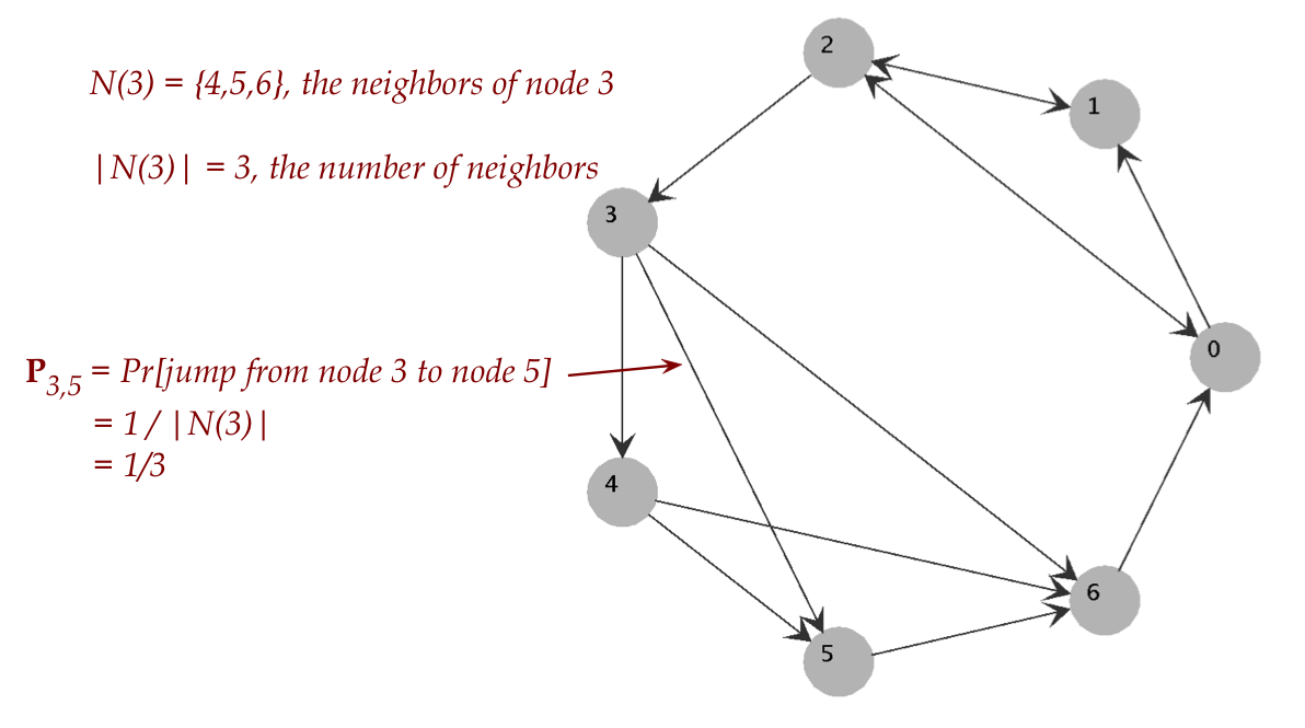
Modeling the web as a graph:
- Each webpage is a node in the graph.
- A directed edge from page i to page j indicates
that page i links to page j.
- Let \(N(i)=\{j: (i,j)\mbox{ is an edge in the graph}\}\)
- That is, \(N(i)\) = the set of neighbors of node i.
In-Class Exercise 10:
Start at this webpage, follow links
to build the graph of the pages labeled 0 through 6.
Write down \(N(i)\) for each node i.
In-Class Exercise 11:
Download PageRank.java,
compile and execute to confirm your graph. You will also need
to download network.txt.
Graph structure:
- We will make some assumptions about the graph
structure (not the original web structure).
- Reachability assumption:
It is possible to start at any node and reach any other node
through link (edge) following.
- Of course, this is not a realistic assumption for the
web and so, we will add links to the graph to
induce reachability.
\(\rhd\)
We will show later how this is done.
- For the moment, let's assume reachability.
Random surfer model:
- Imagine a surfer starting at some node.
- The surfer picks a random link to follow. And repeats this process.
- Thus, the high-level idea is:
    i = initial node
    for k=0 to ...
        j = randomly selected node from N(i)
        i = j
    endfor
- This process of walking around a graph is sometimes called
a random walk on graphs.
- Next, we'll count how often a node is visited
- Suppose we have simulated random surfing for \(t\) steps.
- Let \(v_i(t) = \) the total number of times we land on
node i during steps \(0,\ldots,t\).
In-Class Exercise 12:
Click "start" (which begins at node 0),
and then "next" 10 times, observing the node reached
at each step. Write down \(v_i(10)\) for each node \(i\).
Then, click "run" to watch a longer simulation of
the random walk.
- The number
$$
\frac{v_i(t)}{t}
$$
for some large \(t\) is an estimate of the fraction of time
a random walk (random surfer) spends on page \(i\).
In-Class Exercise 13:
Click "start" and "fast-run", and let it run for a full minute
before clicking on "stop".
The values \(\frac{v_i(t)}{t}\) are printed out.
- Define
$$
\pi_i \eql \lim_{t\rightarrow\infty} \frac{v_i(t)}{t}
$$
and the vector
$$
{\bf \pi} \eql (\pi_1,\pi_2,\ldots,\pi_i,\ldots, \pi_n)
$$
- If we could compute \(\pi_i\) for each page \(i\)
analytically, without simulation, we would have a
a way to rank pages:
\(\rhd\)
The higher \(\pi_i\) is, the higher the rank of page \(i\).
- Then, the page rank algorithm
    Algorithm: pageRank (G)
    Input: a directed, reachable graph G
     1.    π = computePageProbabilities (G)
     2.    sort pages according to πi's
- Page ranks are computed occasionally, based on how the web structure
is assumed to change.
- Given a search query like "Hello world"
    Algorithm: search (s)
    Input: a search query s
     1.    Find subset of pages relevant to s
     2.    Sort subset pages according to πi's
     3.    Report list in order of rank (highest first)
In-Class Exercise 14:
How does one find the subset of pages relevant to a search query?
11.3
The page rank algorithm, part II: an eigenvalue problem
We'll now develop some of the theory to compute \({\bf \pi}\),
the vector of page (node) probabilities:
- First, recall how we defined \({\bf \pi}\):
- Each
$$
\pi_i \eql \lim_{t\rightarrow\infty} \frac{v_i(t)}{t}
$$
which is the long-term fraction of time that the random surfer
spends time on page \(i\).
- \({\bf \pi}\) is merely the vector of these probabilities:
$$
{\bf \pi} \eql (\pi_1,\pi_2,\ldots,\pi_i,\ldots, \pi_n)
$$
- Next, define the transition probabilities
$$
P_{ij} \eql \mbox{ the probability of jumping from i to j}
$$
and the transition probability matrix
$$
{\bf P} \eql
\mat{P_{11} & P_{12} & \ldots & P_{1n}\\
P_{21} & P_{22} & \ldots & P_{2n}\\
\vdots & \vdots & \vdots & \vdots \\
P_{n1} & P_{n2} & \ldots & P_{nn}
}
$$
In-Class Exercise 15:
For our running example, write down the transition probability
matrix. Then, un-comment Section B of the code in
PageRank, compile and execute. Compare your
matrix with the one printed out.
Explain the relationship between the entries of the matrix
and \(N(i)\).
- We claim that
$$
{\bf \pi}^T \eql {\bf \pi}^T {\bf P}
$$
which we will explain below.
- If this were true, we take transposes of both sides:
$$
{\bf \pi} \eql {\bf P}^T {\bf \pi}
$$
- Define the matrix \({\bf A} = {\bf P}^T\).
- Then, we can rewrite as
$$
{\bf A} {\bf \pi} \eql {\bf \pi}
$$
Or, in our more familiar form:
$$
{\bf A} {\bf x} \eql {\bf x}
$$
- Clearly, this makes \({\bf \pi}\) an eigenvector of
the matrix \({\bf A}\).
In-Class Exercise 16:
What is the corresponding eigenvalue?
- Furthermore, if it so happens that \({\bf \pi}\)
is the eigenvector corresponding to the highest eigenvalue,
then we can use the power method.
In-Class Exercise 17:
Un-comment Section C in the code to run the power method.
Examine the code in the power method to confirm that we
are indeed applying the power method. Compare the
resulting probabilities \({\bf \pi}_i\) with the estimates
\(\frac{v_i(t)}{t}\) printed out (after simulating a few minutes).
- We thus have a way to compute the vector \({\bf \pi}_i\)
as a first step towards ranking the pages:
    Algorithm: pageRank (G)
    Input: a directed, reachable graph G
     1.    P = makeTransitionMatrix (G)
     2.    A = PT
     3.    π = powerMethod (A)
     4.    sort pages according to πi's
- The transition matrix is of course
$$
{\bf P}_{ij} \eql \frac{1}{|N(i)|} \;\;\;\; \mbox{whenever
(i,j) is an edge}
$$
- For example:
We have two things remaining to prove:
- Explain why \({\bf \pi}^T = {\bf \pi}^T {\bf P}\).
- Show that \(\lambda=1\) is the largest eigenvalue,
which would make \({\bf \pi}\) the eigenvector that
results from the power method.
11.4
The page rank algorithm, part III: the theory
Why \({\bf \pi}^T = {\bf \pi}^T {\bf P}\):
- Consider the i-th component of \({\bf \pi}\), that is, \(\pi_i\).
- This is the product of \({\bf \pi}^T\) and the i-th column of
\({\bf P}\):
$$
\pi_i \eql \pi_1 {\bf P}_{1,i} + \pi_2 {\bf P}_{2,i} +
\pi_3 {\bf P}_{3,i} + \ldots + \pi_n {\bf P}_{n,i}
$$
- To show that this is true, first define
$$
q_i(t) \eql Pr[\mbox{you land on page i in step t}]
$$
- Then, we'll argue that
$$
q_i(t+1) \eql q_1(t) {\bf P}_{1,i} + q_2(t) {\bf P}_{2,i} +
q_3(t) {\bf P}_{3,i} + \ldots + q_n(t) {\bf P}_{n,i}
$$
Why should this be true?
- Suppose we are on page 1 at time \(t\).
- The probability of getting to page i at \(t+1\) is
the "jump probability" from 1 to i:
$$
Pr[\mbox{go from 1 to i}] \eql {\bf P}_{1,i}
$$
- Similarly, if we are on page \(j\),
$$
Pr[\mbox{go from j to i}] \eql {\bf P}_{j,i}
$$
- Thus, the probability of find oneself on page i comes
from accounting for all possible previous states:
$$
Pr[\mbox{on page i at t+1}]
\eql
\sum_{j} Pr[\mbox{on page j at t}] {\bf P}_{j,i}
$$
- In other words,
$$
q_i(t+1) \eql \sum_j q_j(t) {\bf P}_{j,i}
$$
- Now consider the limit at \(t\rightarrow\infty\):
$$\eqb{
\lim_{t\rightarrow\infty} q_i(t+1)
& \eql &
\pi_i\\
\lim_{t\rightarrow\infty} q_j(t)
& \eql &
\pi_j
}$$
- And so,
$$
\pi_i \eql \sum_j \pi_j {\bf P}_{j,i}
$$
which is the i-th component of
$$
{\bf \pi}^T \eql {\bf \pi}^T {\bf P}
$$
The largest eigenvalue of \({\bf A}={\bf P}^T\):
11.5
The page rank algorithm, part IV: practicalities
We'll address two practical issues:
- What to do about dangling nodes?
- The matrix is very, very large.
Dangling nodes:
- These are pages that don't link to anything.
- Just as bad are subgraphs that cause the random surfer
to loop endlessly within a tiny part of the graph.
In-Class Exercise 19:
Draw an example of a 6-vertex graph with both of the
above problems.
- To address the above problem, we'll use a simple trick.
- At each page, the surfer decides between
- Following one of the outgoing edges, selected randomly.
- Randomly jumping to any node in the whole graph.
- To decide between the two, the surfer uses a biased coin
with \(Pr[\mbox{heads}] = \alpha\).
- If the old transition matrix was \({\bf P}\),
the new transition matrix then becomes
$$
{\bf G} \eql
\alpha
\mat{
P_{11} & \ldots & P_{1n} \\
P_{21} & \ldots & P_{2n} \\
\vdots & \vdots & \vdots \\
P_{n1} & \ldots & P_{nn} \\
}
\plss
(1-\alpha)
\mat{
\frac{1}{n} & \ldots & \frac{1}{n} \\
\frac{1}{n} & \ldots & \frac{1}{n} \\
\vdots & \vdots & \vdots \\
\frac{1}{n} & \ldots & \frac{1}{n} \\
}
$$
In-Class Exercise 20:
Explain why this is true. That is, why is
\({\bf G}_{ij}\) the probability of jumping from
i to j with the new two-step surfing rule?
In-Class Exercise 21:
Why does this two-step rule solve the dangling node problem?
Now for the size problem:
- Let's examine the power method iteration with
\({\bf G}^T\).
- Since \({\bf G}^T\) is a full matrix (every entry is
nonzero), that's a huge number of entries to store.
- However, there is a simplification that works.
- First, write the transpose in terms of \({\bf P}^T\)
$$
{\bf G}^T \eql
\alpha
{\bf P}^T
\plss
(1-\alpha)
\mat{
\frac{1}{n} & \ldots & \frac{1}{n} \\
\frac{1}{n} & \ldots & \frac{1}{n} \\
\vdots & \vdots & \vdots \\
\frac{1}{n} & \ldots & \frac{1}{n} \\
}
$$
- Next, define the vector
$$
{\bf h} \eql \vecfour{1}{1}{\vdots}{1}
$$
- Then we can write the matrix on the right as
$$
\mat{
\frac{1}{n} & \ldots & \frac{1}{n} \\
\frac{1}{n} & \ldots & \frac{1}{n} \\
\vdots & \vdots & \vdots \\
\frac{1}{n} & \ldots & \frac{1}{n} \\
}
\eql
\frac{1}{n}{\bf hh}^T
$$
where, remember, that \({\bf h}^T\) is a single-row matrix.
In-Class Exercise 22:
Show that this is the case.
- Then, we can write
$$
{\bf G}^T \eql
\alpha {\bf P}^T + \frac{(1-\alpha)}{n} {\bf hh}^T
$$
- And the power method iteration becomes
$$\eqb{
{\bf x}^{(k)}
& \eql &
{\bf G}^T {\bf x}^{(k-1)} \\
& \eql &
\alpha {\bf P}^T {\bf x}^{(k-1)}
+ \frac{(1-\alpha)}{n} {\bf hh}^T {\bf x}^{(k-1)} \\
& \eql &
\alpha {\bf P}^T {\bf x}^{(k-1)}
+ \frac{(1-\alpha)}{n} {\bf h} ({\bf h}^T {\bf x}^{(k-1)}) \\
& \eql &
\alpha {\bf P}^T {\bf x}^{(k-1)}
+ \frac{(1-\alpha)}{n} {\bf h}
}$$
where the last simplification comes from
$$
{\bf h}^T {\bf x}^{(k-1)} \eql 1
$$
In-Class Exercise 23:
Why is this last step true? Hint: remember that
\({\bf x}^{(k-1)}\) are probabilities that sum to 1.
What happens when you left multiply by \({\bf h}^T\)?
- Thus, the only real "work" that takes time is
to multiply the matrix \({\bf P}^T\) into the
vector \({\bf x}^{(k-1)}\).
- Here, the matrix \({\bf P}^T\) is very sparse.
In-Class Exercise 24:
Why is \({\bf P}^T\) sparse?
- Fortunately, there are some simple tricks to store
and multiply sparse matrices.
- For example, store each row as a linked list.
\(\rhd\)
Each row will only have a few entries.
In-Class Exercise 25:
Explain how matrix-vector multiplication would work. That is,
write pseudocode to multiply a matrix row represented as
a linked-list into a vector stored as an array.
11.6*
The QR algorithm
So far, we have a method to find one eigenvector: the one
corresponding to the largest eigenvalue
\(\rhd\)
The power method
What about the other eigenvectors?
- It turns out: this is quite a difficult problem.
- It took decades to develop techniques to be able to do this
reliably, and for large matrices.
- There's a variety of quite different techniques today
\(\rhd\)
The subject of numerical linear algebra
- We could easily spend a whole semester on these methods.
- But since we capped off the study of orthogonality with
the QR-decomposition, we'll describe an algorithm based on it.
- The algorithm is quite simple to implement, but
impossibly difficult to intuit.
- What's nice about it: it gives us all the eigenvalues
(and eventually eigenvectors) at once.
The QR algorithm:
- First recall the QR-decomposition: any matrix \({\bf A}\)
with independent
columns can be decomposed into the product
$$
{\bf A} \eql {\bf QR}
$$
where \({\bf Q}\) is orthogonal and \({\bf A}\) is
upper-triangular and invertible.
- Let's describe the steps in the iterative QR algorithm:
- Start by decomposing \({\bf A}\):
$$
{\bf A} \eql {\bf Q}_0 {\bf R}_0
$$
- Then, create a new matrix
$$
{\bf A}_1 \; \defn \; {\bf R}_0 {\bf Q}_0
$$
- Then, do the QR for \({\bf A}_1\)
$$
{\bf A}_1 \eql {\bf Q}_1 {\bf R}_1
$$
- Then, create \({\bf A}_2\)
$$
{\bf A}_2 \; \defn \; {\bf R}_1 {\bf Q}_1
$$
- And so on.
- In pseudocode:
     Algorithm: QRmethod (A)
     Input: a square matrix A with independent columns
     1.   for k=0 to ...
     2.       (Q, R) = QR-decomposition (A)
     3.       A = R Q
     4.   endfor
     5.   return diagonal (A)             // Eigenvalues are on the diagonal
- It turns out that this iteration converges. Let's give the
limiting matrix a name:
$$
\lim_{k\rightarrow\infty} {\bf A}_k \eql {\bf A}^\prime
$$
- Next, define
$$
\mbox{diag}({\bf A}^\prime) \eql
\mbox{ the diagonal entries of } {\bf A}^\prime
$$
- It turns out, quite surprisingly, that:
$$
\mbox{diag}({\bf A}^\prime) \eql
(\lambda_1,\lambda_2,\ldots,...,\lambda_n)
$$
That is, the diagonal entries of \({\bf A}^\prime\) are
the eigenvalues of \({\bf A}\)!
- This is not at all trivial to prove. We will refer to the
text by Olver and Shakiban (Chapter 10) for a proof.
- The iteration only provides the eigenvalues.
- But once we know an eigenvalue \(\lambda\), the
corresponding eigenvector can be found from the RREF, as follows:
- If \({\bf x}\) is the eigenvector corresponding to
\(\lambda\) then
$$
{\bf Ax} = \lambda{\bf x}
$$
- We can write the right side as
$$
{\bf Ax} = \lambda {\bf I} {\bf x}
$$
- Which means
$$
{\bf Ax} - \lambda {\bf I} {\bf x} \eql {\bf 0}
$$
Or
$$
({\bf A} - \lambda {\bf I}) {\bf x} \eql {\bf 0}
$$
- Since we know \(\lambda\), we know the matrix
$$
{\bf B} \eql {\bf A} - \lambda {\bf I}
$$
- Which means, to find \({\bf x}\) we need to solve the equations
$$
{\bf Bx} \eql {\bf 0}
$$
- Which we know how to do quite well.
In-Class Exercise 26:
Review your work in Exercise 5 showing that
\({\bf x}_1=(\frac{1}{\sqrt{2}},\frac{1}{\sqrt{2}})\)
and \({\bf x}_2=(\frac{1}{\sqrt{2}},-\frac{1}{\sqrt{2}})\)
are eigenvectors of \({\bf A}=\mat{2 & 1\\1 & 2}\).
What were the eigenvalues?
Download, compile and execute
QRExample.java
to see the QR algorithm find the eigenvalues.
Note:
- We have described the above algorithm just for completeness, to show
that there are ways of computing a full set of eigenvalues.
- This is not really an "exam" topic or anything critical to
understanding the remaining material.
- The general problem of computing eigenvalues efficiently is
difficult and an advanced topic.