Simulation: An Introduction
Overview of Computation in Biology
Search problems
- Goal: search term or comparison
- Exact match searches:
- Alignment search: e.g., Blast
- Image search/comparison: e.g., microarray databases
Data characterization problems
- Clustering:
- Identify related genes using microarray data.
- Data mining:
- Identify patterns in data.
- Example: pathway extraction in GenMapp
- Phylogenetic tree construction:
Visualization:
Special purpose algorithms:
- Sequence re-construction from DNA sequence data.
- Peptide re-construction from mass-spec data.
- Gene prediction algorithms.
Simulation: (this lecture)
What is Simulation?
Broad definition: A simulation is a computational model of a "process".
More specific definition:
- A simulation will typically have many small interacting
elements with cause-event relationships.
=> reflects real-world elements as closely as possible
- Simulations are usually stochastic
=> some randomness in system
- The goal is usually to measure macro-properties based on
the interactions of the small elements.
Example:
- Consider this problem: Flip a coin 10 times. What is the
probability that exactly 2 "heads" are observed?
- Analytical solution:
- Pr[exactly 2 heads] = n*(n-1)*2-(n+1) for
n flips.
- Thus, for 10 flips:
Pr[exactly 2 heads] = 10*(10-1)*2-11 = 0.04
- Note: we can write a (Java) program to compute this:
   prob = n * (n-1) * Math.pow (2, -(n+1));
   System.out.println (prob);
Is this a simulation?
- Consider this program instead:
   numSuccesses = 0;

   // Repeat experiment several (numTrials) times
   for (int i=0; i < numTrials; i++) {

     // Flip coin n times.
     numHeads = 0;

     for (int j=0; j < n; j++) {
       boolean isHeads = randomCoinFlip ();
       // Count number of heads.
       if (isHeads)
         numHeads ++;
     }

     // Experiment is a success if we get exactly 2 heads.
     if (numHeads == 2)
       numSuccesses ++;
   }

   // At end, estimate probability
   prob = numSuccesses / numTrials;
   System.out.println (prob);
This is a simulation.
Characteristics of a simulation:
- System (process) evolution.
- Randomness.
- Difficult to compute analytically.
- Repeatable, verifiable.
- Parametrizable.
Types of simulation:
- Continuous:
- State variables are continuous.
- Usually based on differential equations.
- Discrete or discrete-event:
- State variables may be discrete or continuous.
- System evolves from event to event.
Exercise:
Find two examples of biology-related simulation on the web.
See if you can categorize them into "continuous" or "discrete".
Anatomy of a Discrete-Event Simulation:
Random Walk Example
Demo: 1-D random walk
General structure of 1-D random walk:
- Collection of "states" ordered left to right:

Here, the states are numbered 1, ..., n
- Think of a "token" that represents the current state:
- At each state, there are "jump probabilities" specifying
motion of the token to the left or right.
Thus, in this example, there's a propensity to drift rightwards.
- The token starts in some state and at each step jumps
randomly (according to jump probabilities) to a neighboring state.
- Let Xk = state after k jumps.
- Typical questions of interest:
- What is Pr[Xk = i]?
- What is limk -> infinity Pr[Xk = i]?
- What is E[Xk]?
Why study random walks?
Types of random walks:
Simulating a random walk:
- Suppose we want to estimate Pr[gambler is ruined]? above.
- Simulation parameters:
- p = 0.4
- Start with fortune = n/2.
- First, consider simulating a single walk:
Algorithm: gamblerRuin (N)
Input: the highest state
1.  state = N/2
2.  reachedZero = false
3.  reachedN = false

4.  while not (reachedZero or reachedN)
5.    if coinFlip(0.4)
6.      state = state + 1     // Go to state + 1
7.    else
8.      state = state - 1     // Go to state - 1
9.    endif

10.   // See if game is over.
11.   if state == 0
12.     reachedZero = true
13.   if state == N
14.     reachedN = true
15. endwhile

16. return reachedZero

Output: whether random walk was absorbed at the left
- Now, to get a proper estimate we'll have to repeat this
several times:
Algorithm: estimateRuin (N)

1.   numRuins = 0
2.   for i=1 to numTrials
3.     ruined = gamblerRuin (N)
4.     if ruined
5.       numRuins = numRuins + 1
6.     endif
7.   endfor
8.   return numRuins / numTrials
Simulation Example: Epidemiology
Epidemiological questions of interest:
- What is the rate of infection (new infections/day)?
- What percent of population gets infected?
- How effective are vaccination policies? e.g.,
- Flu: vaccinate school kids, medical workers
- Smallpox: vaccinate medical/rescue workers, police, military
Modeling approaches:
- Differential equations:
- Write down a differential equation that expresses key
characteristics of system.
- Solve analytically or numerically.
- Simulation:
- Build detailed computational model.
- Implement simulation.
- Run simulations to extract statistics.
Differential-equation modeling of epidemics:
- Consider a population of size N.
- Let U(t) = number of uninfected people.
- Let I(t) = number of infected people.
- Modeling assumption: the rate of new infections depends on:
- I(t)
=> the higher I(t), the more the chance of
infectious contact
- U(t)
=> the higher U(t), the higher the number of
susceptible people.
- Thus, [I(t+s) - I(t)] / s = (constant) U(t) I(t).
- Alternatively:
[U(t+s) - U(t)] / s = - (constant) U(t) I(t).
- Differential equation: U'(t) = - b U(t)I(t).
- Turns out: can be solved analytically in some cases.
Advantages of differential-equation modeling:
- Well-known solution techniques (over 300 years of mathematics).
- Easily verifiable (mathematical proofs).
- Forces attention on key characteristics.
- Analytic solutions provide insight (e.g., exponential
growth vs. linear growth).
Limitations of differential-equation modeling:
- Only simple cases are tractable.
- It's hard, if not impossible, to model:
- Randomness, e.g., probabilistic contact
- Individual behavior, e.g., individuals that use history of
observed behavior
- Non-linear effects, e.g., vaccination policies
- Spatial effects, e.g., contact in spatial vicinity
A simple simulation model:
- "Agents" (people) roam about randomly on a 2D grid
(modeling contact).
- Infections occur between an uninfected agent and infected
agent in the same cell (spatial effects).
- Goal: estimate number of infected agents at end of simulation.
Demo
A more complex simulation model:
- Agent characteristics:
- Families with different sizes.
- Age distributions and age-based susceptibility.
- Spatial characteristics:
- Contact in workplaces, schools, malls, hospitals.
- Randomness in time spent, number of contacts.
- Disease characteristics:
- Injection model: how does it start?
- Progression parameters: incubation, immunity, contagiousness, susceptibility.
- Infection events: workplace events, age-based, school-based.
- Policy characteristics:
- Vaccination policies: forced vaccination, inducements, school-based.
- Information distribution: monitoring, health-alerts.
Demo (work in progress)
Simulation Example: Protein Folding
Protein folding overview:
- Why: protein folds = protein function
- Estimate: about 3000 different types of folds
=> currently 300 folds in PDB
- Computational goal: given protein sequence, predict folds
- Note: a single protein can have multiple domains, each with
its own important fold/function.
One computational approach:
- Model force/energy interactions at atomic or small-molecule level.
- Each configuration (fold) has an associated (potential) energy.
- Computational goal: find minimal energy configuration.
An illustrative example: 2D protein folding:
- Use 2D grid to represent space.
- Each amino acid occupies one cell.
- Interaction between neighboring cells.
- Protein must occupy contiguous cells.
- Energy computation:
- Specify amino-amino energies in a table.
- Total energy = sum of all neighboring amino-amino energies.
Exercise:
Compute the energy of the above fold.
- Solution procedure:
- Start with a random guess (fold).
- Modify fold to see whether a "better" fold can be found.
- Iterate until low-energy configuration is found.
Demo
Why it's a hard computational problem:
- Iterative folding gets "stuck" at local minima.
- Astronomically large number of possible folds.
Solution approaches:
- Parallel/super computing: e.g., IBM's
BlueGene project.
- Distributed computing: e.g.,
Folding@Home project.
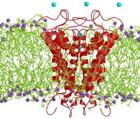
Membrane Simulation
Membrane simulation goals:
- Modeling of membrane structure and formation.
- Modeling of transport through membranes.
- Modeling of membrane protein interactions.
Why membranes?
- Lot of molecular chemistry (signalling etc) occurs at membranes.
- Estimate: 30% of proteins involved in some membrane function.
- Common target for drugs.
Demo: simple membrane formation model (compare)
Simulating Chemistry
Differential equation models:
- Consider a chemical A that transforms into B:
- The rate at which A transforms into B depends
on the number of A molecules:
dB/dt = k A
- Similarly, dA/dt = -k B
(because A + B = constant)
- For a reaction A + B <=> C, the equations are
- dC/dt = k AB
- dA/dt = - k AB
- dB/dt = - k AB
- Solve using standard diff-eq methods or packages.
- Solution: equilibrium quantities.
Stochastic models:
- Consider the reaction A + B <=> C.
- Let
nA = number of A molecules
nB = number of B molecules
nC = number of C molecules
- At any time, the current "state" of the system is
given by (nA, nB, nC)
- Define state transition probabilities:
- Here, p and q may depend on the state.
- To solve: run simulation and compute statistics.
- Possible to extract chemical dynamics from simulation.
Modeling catalysis
- Consider the following reaction:

- We can model the reaction as follows:
- At each step (e.g., a nanosecond), the forward reaction is:
A = A - x
B = B - x
C = C + 2x
- Here, x is a small quantity (fixed number of molecules).
- Reaction proceeds only if ABD > threshold.
Simulation and Origin-of-Life Theories
Let's start with some perspective:
| Event | How many years ago |
| Big bang | 20,000,000,000 |
| Planets | 5,000,000,000 |
| Life | 3,500,000,000? |
| Photosynthesis | 2,500,000,000 |
| First eukaryote | 1,500,000,000 |
| Multicellular | 1,000,000,000 |
| Modern man | 200,000 |
| ? | ? |
| Beginning of semester | 0.25 |
| Beginning of lecture | 0.000171 |
Exercise:
Fill in the question marks in the above table with something
interesting that's related to biology.
Current favorite theory:
- Early earth (post big-bang) had no organic compounds.
- Bombardment by cosmic rays, lightning, UV etc created simple
organic compounds.
=> the "primitive soup"
- Primitive soup contained amino acids, nucleic acids.
- RNA happens!
- Then came DNA, Krebs cycle, protein machinery etc.
But ...
- Which came first: proteins or nucleic acids?
- Proteins first theory: nucleic-acid structures were
facilitated by proteins.
- Naked genes theory: DNA first replicated by
itself, proteins were created later.
- What are the chances that a complex molecule like RNA be constructed randomly?
Evidence:
- The Miller experiment: bombard non-organic soup with
lab-lightning
=> produces organic compounds.
- Variants of Miller experiment: production of amino acids,
bases, sugars.
- Proteinoids: artificial creation of proteins
- Heat amino acids (with some substrate) and cool
=> randomly linked amino acids
- Heat amino acids with some types of clay
=> crystalline structure in clay forces binding of acids.
- Lab evidence: proteinoids can catalyse some reactions.
RNA-world theory: "First there was RNA"
- Self-splicing RNA (example: fungal mitochondria)
- Ribozymes: RNA that can act as an enzyme (example: ribonuclease P)
- Problems with "RNA-world":
- What is the likelihood of
random creation of RNA?
- RNA is not very stable.
- Can simulation help in answering the question: why?
=> was Life an accident?
Autocatalysis theory:
Demo
Cellular Automata and Von Neumann's Quandary
Cellular Automata:
- What is a cellular automaton?
- An infinite cellular space - usually a 2D grid:
- Set of states, e.g, S = { empty, A, B, C, D }.
- Initially each cell is in one of the states:
- System evolves in time-steps.
- At each step, "rules" are applied to generate the next state
for each cell, e.g.,
- State-transition rules:
- A neighborhood for each cell is defined, usually one of
- 4-neighborhood (N, S, E, W).
- 8-neighborhood (N, S, E, W, NE, NW, SE, SW).
- The next state of a cell depends on its current state and the
current state of its neighbors.
- All cells change state at the same time.
- The rules are sometimes called the "physics" of the system.
In-Class Exercise 12.3:
Search the web for applets that simulate the Game of Life and examine
what happens to the following patterns. Run each pattern for a few
time steps (generations).
- The Blinker.
- The Block.
- The Glider.
- The R-pentonimo.
The Game of Life:
- A cellular automaton with only two states: on and off.
- Devised in 1970 by John Horton Conway.
- Rules:
- Uses 8-neighborhood.
- Rule 1 (birth): if a cell has exactly 3 neighbors
"on", its next state is "on".
- Rule 2 (status-quo): if a cell has exactly 2
neighbors "on", its next state is its current state.
- Rule 3 (death): In all other cases, the next state is "off".
- A generalization: k-Game-of-Life
- Birth rule: if a cell has exactly k neighbors "on", its
next state is "on".
- Status quo rule: if a cell has exactly k-1 neighbors "on".
- Death rule: all other values.
- k = 3 in the Game-of-Life.
- Interesting observation:
- If k > 3: too much growth (chaos).
- If k < 3: too little growth (empty space).
- k = 3 is "optimal for life".
Von Neumann's quandary:
- Problem: to prove (mathematically) that self-reproduction is
possible.
- First attempt: the kinematic model (robots):
- Can a robot reproduce, i.e., assemble a copy of itself (that can later reproduce) from a blueprint?
- The blueprint problem: can a blueprint contain itself?
- Second attempt: cellular automaton.
- Trivial vs. non-trivial reproduction in cellular worlds:
- Trivial reproduction: the Blinker in the Game of Life.
- Von Neumann's criteria for non-trivial reproduction: a
cellular automaton that:
- Can embed a Universal Turing machine (i.e., can compute anything)
- Can embed a Universal Constructor (i.e., can build from a blueprint).
- Reproduce itself entirely, including blueprint.
- Von Neumann (with others) showed that it was possible: by constructing a
cellular automaton exhibiting non-trivial self-reproduction:
- 29 states per cell and 200,000 cells.
- The "creature" contained a "tape" with instructions (blueprint), and a
"constructor arm".
- Another part of the cellular creature contained a universal
Turing machine.
- Solution of the blueprint problem: the blueprint was
"photocopied" into the offspring.
- Reproduction occurs in two phases:
- Build the offspring by reading (interpreting) the blueprint.
- Copy over the blueprint into the offspring (without interpreting).
Other developments in cellular automata:
- The Game-of-Life can support computation (and it's believed) self-reproduction.
- Simpler non-trivial self-reproducing cellular automata have
been found
=> all use "blueprint copying".
(Example)
- Cellular automata have become a field of study with attempts
to build "metabolic" creatures (that grow, age, evolve etc).
Intriguing questions and comparison between cellular automata and
our "wet" world:
- Question: Does the physics/chemistry support
"self-reproducing life"?
| Cellular world |
Yes.
e.g, Von Neumann's example. |
| Wet World |
Yes. |
- Question: Does the physics also support trivial reproduction?
| Cellular world |
Yes.
Game-of-Life's Blinker |
| Wet World |
Yes.
Crystalline growth. |
- Question: Does non-trivial reproduction use the
2-step blueprint model?
| Cellular world |
Yes.
All examples |
| Wet World |
Yes.
DNA replication and interpretation. |
- Question: Is evolution supported?
| Cellular world |
Yes.
In some models. |
| Wet World |
Yes.
|
- Question: Is spontaneous occurrence of "life" possible?
| Cellular world |
Not known. |
| Wet World |
Current belief: Yes. |
- Question: Is uncontrolled chaotic growth ("grey goo") possible?
| Cellular world |
Yes.
Game-of-Life's R-pentonimo |
| Wet World |
? |
- Question: Do the elements of self-reproduction also
support computation?
| Cellular world |
Yes.
Many examples |
| Wet World |
Yes.
(next section) |
