Examples of networks:
For comparison, consider
this representation of the internet (Approximately 1.3 million nodes)
General questions about networks:
- What are fundamental properties of networks?
- How are biological networks different from other types of
networks?
- Do properties of networks explain higher-level phenomena?
Overview of lecture:
- Study networks in an abstract sense.
- Identify and explain fundamental properties.
- Describe some aspects of an emerging "science of networks".
Exercise:
What do the terms "Friendster", "Kevin Bacon" and "Six degrees"
have in common?
Exercise:
Use
Star-links to:
- find the Bacon number of a GW-alum.
- find two names that are connected by at least three links.
Exercise:
What does the term Erdos number mean?
Graph theory
Informal definition:
- A graph is a mathematical abstraction used to represent
"connectivity information".
- A graph consists of vertices and edges that
connect them, e.g.,
- It shouldn't be confused with the "bar-chart" or "curve" type
of graph.
Formally:
- A graph G = (V, E) is:
- a set of vertices V
- and a set of edges E = { (u, v): u and v are vertices }.
- Two types of graphs:
- Undirected graphs: the edges have no direction.
- Directed graphs: the edges have direction.
- Example: undirected graph
- Edges have no direction.
- If an edge connects vertices 1 and 2, either
convention can be used:
- No duplication: only one of (1, 2) or (2, 1)
is allowed in E.
- Full duplication: both (1, 2) and (2, 1)
should be in E.
- Example: directed graph
- Edges have direction (shown by arrows).
- The edge (3, 6) is not the same as the edge (6,
3) (both exist above).
Depicting a graph:
- The picture with circles (vertices) and lines (edges) is
only a depiction
=> a graph is purely a mathematical abstraction.
- Vertex labels:
- Can use letters, numbers or anything else.
- Convention: use integers starting from 0.
=> useful in programming, e.g. degree[i] = degree
of vertex i.
- Edges can be drawn "straight" or "curved".
- The geometry of drawing has no particular meaning:
Some basic definitions (for undirected graphs):
- Degree of a node
the number of edges incident to it.
- Path: a sequence of vertices in which successive
vertices have an edge between them.
- Connectivity: two vertices are connected if there is a
path that includes them.
- Component: A subgraph is a subset of vertices together with the
edges from the original graph that connects vertices in the subset.
Example:
Some characteristic measures:
- Degree distribution: how many nodes have degree=1, how
many have degree=2, ... etc.
Consider this example:
In above example:
| 2 vertices with degree=1: |
6, 7
|
| 3 vertices with degree=2: |
0, 1, 4, 5
|
| 2 vertices with degree=3: |
2, 3
|
Thus, the degree distribution is: {2, 3, 2}
- Average Shortest-Path (SP) length:
compute this with the following procedure
- For each pair of vertices: compute length of shortest path
connecting them.
- Take the average over all vertex-pairs.
For above example: average = 2.06
- Cluster coefficient: compute as follows
- For each vertex, compute its clustering:
- Identify neighbors.
- Identify the number of connections amongst neighbors.
- If m=#neighbors, divide clustering by (m-1)*m/2.
- Average over all vertices.
For the above example: 1.75
Exercise:
Build the connectivity graph for the class. Compute the measures above.
The field of graph theory
History:
Some famous problems in graph theory:
- Euler tour: A cycle that traverses all edges exactly
once (but may repeat vertices).
Known result: Euler tour exists if and only if all vertices have
even degree.
- Hamiltonian tour: A cycle that traverses all vertices
exactly once.
Known result: testing existence of a Hamiltonian tour is (very) difficult.
- The Four-Color problem: given a map of regions, at most
four colors are needed to color so that no two adjacent regions
have the same color.
Exercise:
How many colors are needed for the 8-node graph above?
- Traveling Salesman Problem (TSP): which tour of the
vertices has the least overall length?
Applications of graph theory:
- Fundamental mathematical construct to represent "connectivity".
- Appears in thousands of problems.
- Source of many classic problems: traveling salesman, routing,
spanning trees.
- Many "graph-structured" applications: networks,
transportation-systems, electronic circuits, molecules.
Graph theory as a source of computer science theory:
- Many important algorithms.
- Key to understanding algorithm design and analysis.
- Simple to describe, yet perplexing:
- Euler tour: easy problem.
- Hamiltonian tour: hard problem.
The field of graph theory:
- Large area of mathematics:
- Analysis of general graphs.
- Analysis of special types of graphs.
- Many classic problems
e.g., the four-color theorem.
- Optimization problems based on graphs,
e.g., shortest-paths.
- Graph algorithms: an area in computer science.
- Rich source of algorithms, theory, insight.
- Useful algorithms used in many applications
(e.g., in a compiler).
Random graphs
Consider this procedure to generate a random graph:
- Draw n vertices.
- Consider each possible pair of vertices in turn:
- For each such pair, flip a coin.
- If heads, place an edge between these vertices.
Exercise:
Split into groups of 4 or 5. Generate a random graph with 10 nodes
using coin flips.
Exercise:
Suppose we use a coin where Pr[heads] = 0.1.
Will we get more or fewer edges than with a fair coin?
Parametrized random graphs:
- Parameter: 0 < p < 1 (density)
- Use a coin such that Pr[heads] = p to generate the
graph.
Exercise:
Split into groups of 4 or 5. Generate a random graph using p = 0.1.
Connectivity:
- Clearly, if p is small, we might have multiple components
(disconnected graph).
- Examples (using graph tool).
- Major result (Erdos and Renyi):
- If p < 1/n, the graph is almost always disconnected.
- If p >= log(n)/n, the graph is almost always connected.
- If 1/n < p < log(n)/n, the graph is dominated by
a giant component.
Other properties:
- Average path length is small: about log(n).
- Cluster coefficient is very small: less than 1.
Exercise:
Can you create a graph where the average shortest-path is
quite long?
The small world phenomenon
Small world phenomenon:
- Stanley Milgram's experiment (1967).
- Path length:
For any two random persons, there exists six people to connect
them.
=> short path lengths.
- Cluster coefficient:
your friends are friends amongst themselves
=> high cluster coefficient.
Observation: the standard random graph does not model "small
world".
The Watts-Strogatz random model:
- Two parameters:
- p: the probability of re-arrangement.
- k: the number of "ring" neighbors.
- Start with a ring.
- Each node is connected to k successive neighbors.
- For each edge in turn:
- Flip a p-biased coin.
- If heads, replace edge with a random edge from one of its
nodes to a random other node.
Examples: (demo)
Properties:
Examples of small world graphs.
|
|
|
Lactual
|
Lrandom
|
Cactual
|
Crandom
|
|
Film actors
|
3.65
|
2.99
|
0.79
|
0.00027
|
|
Power grid
|
18.7
|
12.4
|
0.080
|
0.005
|
|
C. elegans
|
2.65
|
2.25
|
0.28
|
0.05
|
|
(From http://www.santafe.edu/sfi/publications/Bulletins/bulletinFall99/workInProgress/smallWorld.html)
|
|
Applications:
- (Biology) Modeling of disease epidemics.
- (Epidemiology) Efficacy of needle-exchange programs (AIDS prevention):
- Used needle = random link.
- Removal of discarded needles: reduces chances of disease
percolation (epidemic).
- (Economics) Modeling of fads, momentum investing.
- (Business) Organizational hierarchy (Toyota example).
- (Commercial) meetup.com, friendster.com, tribe.com, linkedin.com
Power-law graphs
Exercise:
Which function is "smaller" for fixed k: f(n) = e-kn
or g(n) = n-k?
Consider the degree distribution of a graph:
- Let fi = number of vertices with i edges.
- One can show that for random graphs, fi is
proportional to e-a*i (for some constant a).
- A power-law graph is a graph in which
fi is proportional to i -k (for some constant k).
Examples:
- A random (Erdos-Renyi) example (demo).
- E-Coli gene regulation graph (demo).
- Internet, among many other real data sets.
Implications:
- Random graphs have very few high-degree nodes.
- Power-law graphs have some high-degree nodes.
- Robustness implications:
- A random removal of nodes can disconnect a random network.
- Power-law graphs are more resistant to random removals.
- Power-law graphs are extremely sensitive to targeted removals.
=> Consider what happens when you remove the high-degree nodes.
- Biological implications:
- High-degree nodes: genes involved in regulating many others (bookkeeping).
- Robustness necessary to support mutation/evolution.
Network motifs
A graph or network motif is a small localized sub-structure in a graph.
Notation: TF = Transcription Factor
Example: Feed-Forward (FF) loop motif:
- A Feed-Forward loop has three elements:
- Two kinds of FF's:
- Data from E Coli:
- FF-loops occur more frequently than in random graphs.
- 85% of FF loops are coherent.
Example: Single-Input Module (SIM) motif:
- One TF regulates many genes.
- Data from E Coli:
- 24 such motifs
- Large SIM's, that occur in E Coli, are highly unlikely in random graphs.
Motif function:
Coordination:
- Coordination is needed to achieve a larger, higher-level function.
- In a computer, there is an explicit module that controls the
sequence of events:
- But in biological systems? Is there a central controller?
Network dynamics
Static properties of graphs:
- Examples: connectivity, degree distribution, cluster coefficient.
- Limitations:
- Static properties don't explain behavior.
- Static properties may not help with small networks.
Boolean networks: a model of network dynamics
- Start with a directed graph.
Example:
- Each vertex is in one of two states:
- "On" (gene is turned on)
- "Off" (gene is turned off)
- Use 1 for "on" and 0 for "off".
- Example: suppose only node 5 is "on":
- Example: nodes 0, 1, 2, 5 are "on":
- The state of the network is itself a number:
- In the first state above: state = 000001
=> binary value 1
- In the second state above: state = 111001
=> binary value 57
- The evolution of a boolean network:
- At each step: apply "rules" to current state to
get next state.
- Repeat.
- What are the "rules"?
- A rule specifies how inputs to a node affect the next state.
- Thus, for vertex v, suppose Sv is the
current state.
- Suppose v has k upstream neighbors with current states
S1,...,Sk.
- The next state for v is some function
S'v = F (Sv, S1,...,Sk).
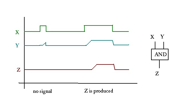
- Two types of commonly-used rules:
- Unweighted-threshold:
|
S'v = 1,
|
|
if (S1 + ... + Sk) - t > 0.
|
|
S'v = 0,
|
|
if (S1 + ... + Sk) - t < 0.
|
|
S'v = Sv,
|
|
if (S1 + ... + Sk) - t == 0.
|
- Weighted-threshold: associate a weight Wi with each incoming edge
|
S'v = 1,
|
|
if (W1 S1 + ... + Wk Sk) - t > 0.
|
|
S'v = 0,
|
|
if (W1 S1 + ... + Wk Sk) - t < 0.
|
|
S'v = Sv,
|
|
if (W1 S1 + ... + Wk Sk) - t == 0.
|
- Weighted-thresholds model gene down-regulation:
- Use positive edge weight (Wi = 1) for up-regulation.
- Use negative edge weight (Wi = -11) for down-regulation.
Exercise:
Consider the example from earlier:
- How many possible states are there for this graph?
- Assume t = 0 and use the unweighted rules.
- Start with the state in which only vertex 5 is "on".
What is the next state? And the state after that? And after that?
- Do the same for the case t = 1.
The state graph:
- Recall: each state of the network is a number.
- If there are n vertices, there are 2n
possible states.
- The states are numbered States = {0, 1, ..., 2n-1}.
- Build a graph, the state graph,
with vertices {0, 1, ..., 2n-1}.
- For each state S in States:
- Apply rules to compute next state S' of S.
- Place an edge from S to S' in the state graph.
Exercise:
Consider this example:
- How many possible states are there for this graph?
- Assume t = 0 and use the unweighted rules.
- Compute the state graph. What do you notice?
Attractors and basins:
- In applying the rules, you can get "stuck" in a state:
=> the next state is the same.
- Such states are called attractors.
- Since there is only one outgoing edge for each state (in the
state graph), each state must either go to itself or another one.
- For an attractor state S, let B(S) be the
set of states that "lead" to it.
=> called the Basin of S.
Exercise:
What are the attractors and basins for the above 3-vertex example?
An application to yeast cell-cycle:
(Source: F.Li et
al. The yeast cell-cycle is robustly designed).
- A simplified model of key proteins in the yeast cell-cycle:
- 11 vertices.
- Weighted-threshold model: t = 0.
- Green arrows: up regulation (weight = 1).
- Red arrows: down regulation (weight = -1).
- State graph has 211 = 2048 vertices.
- Part of the state graph showing a major attractor:
- The results show that the most likely path is through a
sequence of states corresponding to the cell cycle: G1, S, G2, M and
back to G1.
- Significance:
- The network dynamics explain the cell cycle.
- The simple interactions of "dumb" elements in a
network can create higher-level complexity.
Complexity
Exercise:
Consider, in general, what happens for different values of the
threshold t:
- What if t is too high?
- What if t is too low?