Biologically-Inspired Algorithms

Preliminaries: What is a Graph?

Informal definition:

A graph is a mathematical abstraction used to represent "connectivity information".

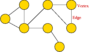
A graph consists of vertices and edges that connect them, e.g.,

It shouldn't be confused with the "bar-chart" or "curve" type of graph.

Formally:

A graph G = (V, E) is:
- a set of vertices V
- and a set of edges E = { (u, v): u and v are vertices }.
Two types of graphs:
- Undirected graphs: the edges have no direction.
- Directed graphs: the edges have direction.
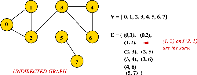
Example: undirected graph
- Edges have no direction.
- If an edge connects vertices 1 and 2, either convention can be used:
  - No duplication: only one of (1, 2) or (2, 1) is allowed in E.
  - Full duplication: both (1, 2) and (2, 1) should be in E.
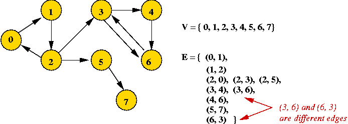
Example: directed graph
- Edges have direction (shown by arrows).
- The edge (3, 6) is not the same as the edge (6, 3) (both exist above).

Depicting a graph:

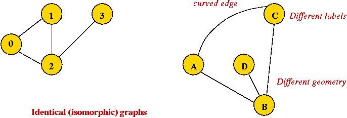
The picture with circles (vertices) and lines (edges) is only a depiction
=> a graph is purely a mathematical abstraction.
Vertex labels:
- Can use letters, numbers or anything else.
- Convention: use integers starting from 0.
  => useful in programming, e.g. degree[i] = degree of vertex i.
Edges can be drawn "straight" or "curved".
The geometry of drawing has no particular meaning:

Exercise: What is the maximum number of edges in an undirected graph with n vertices? What is this number in order-notation?

Paths:

A simple path does not repeat any vertices (and therefore edges) in the sequence.

A cycle is a simple path with the same vertex as the first and last vertex in the sequence.

Euler tour: A cycle that traverses all edges exactly once (but may repeat vertices).

Known result: Euler tour exists if and only if all vertices have even degree.

Hamiltonian tour: A cycle that traverses all vertices exactly once.

Known result: testing existence of a Hamiltonian tour is (very) difficult.

Euler path: A path that traverses all edges exactly once.

Hamiltonian path: A path that traverses all vertices exactly once.

Why are graphs important?

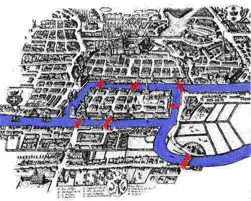
History:
- Maze-searching.
- Euler's crossing problem: the Konigsberg bridges
  How to cross each bridge just once and return to starting point?
Applications:
- Fundamental mathematical construct to represent "connectivity".
- Appears in thousands of problems.
- Source of many classic problems: traveling salesman, routing, spanning trees.
- Many "graph-structured" applications: networks, transportation-systems, electronic circuits, molecules.
Applications in Biology:
- Phylogenetic trees.
- Pathway databases.
- Genetic networks.
Source of theory:
- Many important algorithms.
- Key to understanding algorithm design and analysis.
- Simple to describe, yet perplexing:
  - Euler tour: easy problem.
  - Hamiltonian tour: hard problem.

Optimization Problems

What are they?

An optimization problem has "input" and a "measure"
=> different solutions possible, each of different value
=> Goal: find the "best" solution.

The "measure" is sometimes called an objective function.

Some problems have constraints: not all potentials solutions are "acceptable".

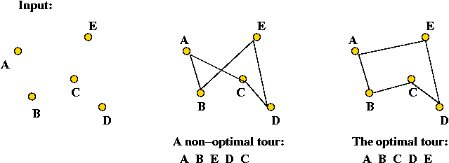
Example: the Travelling Salesman Problem (TSP)

Input: a collection of points (representing cities).
Goal: find a tour of minimal length.
Length of tour = sum of inter-point distances along tour
Details:
- Input will be a list of n points, e.g., (x₀, y₀), (x₁, y₁), ..., (x_n-1, y_n-1).
- Solution space: all possible tours.
- "Cost" of a tour: total length of tour.
  => sum of distances between points along tour
- Goal: find the tour with minimal cost (length).
Note: strictly speaking, we have defined the Euclidean TSP.
=> There is also a graph version that we will not consider
Applications:
- Logistics: trucking and delivery problems.
- Machine operation (e.g., drilling a collection of holes)

Exercise: For an n-point TSP problem, what is the size of the solution space (i.e., how many possible tours are there)?

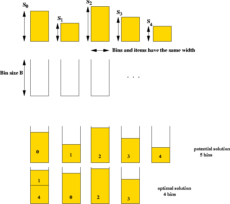
Example: the Bin Packing Problem (BPP)

Input: a collection of items and unlimited bins.
Goal: pack the items into as few bins as possible.
Details:
- Input is a list of n integer bin sizes s₀, s₁, ..., s_n-1 and an integer bin size B.
- Solution space: all feasible packings
  => all assignments of items to bins such that no bin overflows. (A constraint).
  => sum of sizes of items assigned to each bin is at most B.
- Goal: find the assignment that uses the fewest bins.
- Note: assume s_i < B.
Alternate description:
- Item sizes: s₀, s₁, ..., s_n-1 where s_i < B.
- Define the assignment function:
  
  d_ij = 1,
  0, if item i is placed in bin j
  otherwise
- B = bin size.
- Goal: minimize k, the number of bins
  such that:
  1. For each j, s₀d_ij + ... + s_n-1d_ij < B (all items assigned to bin j fit into the bin)
  2. For each i, d_ij + ... + d_ij = 1 (each item is assigned to a bin)

Exercise: Consider the following Bin Packing problem: there are three items with sizes 1, 2 and 3 respectively, and a bin size of 6. Enumerate all possible assignments.

Example: Quadratic Programming Problem

Input: n coefficients a₀, a₁, ..., a_n-1.
Goal: minimize a₀x₀² + a₁x₁² + ... + a_n-1x_n-1².
Constraint: x₀ + ... + x_n-1 = K
Here, each x_i is real-valued.
Example:
Minimize 3 x₀² + 4 x₁²
Such that x₀ + x₁ = 10

Types of optimization problems:

The Quadratic Programming problem is very different from both TSP and BPP.
TSP and BPP are similar is some structural respects.
Two fundamental types of problems:
- Discrete optimization problems: finite or countable solution space.
  => usually finite number of potential solutions.
- Continuous optimization problems: uncountable solution space
  => variables are real-valued.
Examples:
- Discrete: TSP, BPP
- Continuous: Quadratic Programming problem.
We will focus on discrete optimization problems.

Problem Size and Execution Time

Problem size:

Typically, the "size" of a problem is the space required to specify the input:

Example: TSP
=> For an n-point problem, space required is: O(n).

Example: BPP
=> For an n-item BPP, O(n) space is required.

Non-Euclidean TSP

Recall: a graph is given
=> required to use only edges in the graph.
A graph with n vertices can have O(n²) edge
=> O(n²) space required for input.

Consider this TSP example:

Input: "The points are n equally spaced points on the circumference of the unit circle".
How much space is required for an input of 10-points? For 1000-points?
=> O(1) !

The above example is not general
=> we need O(n) space (worst-case) to describe any TSP problem.

Terminology: instance

A problem instance is a particular problem (with the data particular to that problem).
Example: TSP on the 4 points (0, 1), (0.5, 0.6), (2.5, 3.7) and (1, 4).
=> an instance of size 4.
Another instance: TSP on the 5 points (0, 1), (0.5, 0.6), (2.5, 3.7), (1, 4) and (6.8, 9.1).
=> an instance of size 5.

Execution time of an algorithm:

What we expect of an algorithm:
- An algorithm is given its input and then executed.
- The algorithm should produce a candidate solution or report that no solutions are possible.
Example: TSP
- An algorithm is given the set of input points.
- The algorithm should output a tour after execution.
Example: BPP
- An algorithm is given the item sizes and bin size as input.
- The algorithm should output an assignment
  (Or report that some items are too large to fit into a bin).
Output size:
- Example: TSP
  - Output is a tour
    => O(n) output for n points.
- Example: BPP
  - Output is an assignment.
  - If assignment is specified as the function
    
    d_ij = 1,
    0, if item i is placed in bin j
    otherwise
    
    then output could be as large as O(n²).
Execution time:
=> Total execution time includes processing input and writing output.

Consider these two algorithms for TSP:

Algorithm 1:
1. Initially the set P = {0, ..., n-1 } and the set Q is empty.
2. Move 0 from P to Q.
3. Repeat the following until P is empty:
  - Suppose k was the point most recently added to Q.
  - Find the point in P closest to k and move that to Q.
4. Output points in the order in which they were added to Q.
Algorithm 2:
1. Generate a list of all possible tours and place in an array (of tours).
2. Scan array and evaluate the length of each tour.
3. Output the minimum-length tour.

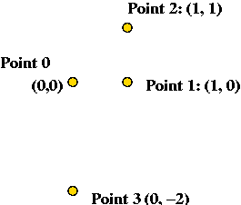
Exercise: Consider the following 4 input points: (0,0), (1,0), (1,1) and (0,-2).

Show the steps in executing each algorithm on this input.

What is the complexity (execution time) of Algorithm 1 on an input of size n?

What is the complexity of Algorithm 2 on an input of size n?

Polynomial vs. exponential complexity:

An algorithm has polynomial complexity or runs in polynomial time if its execution time can be bounded by a polynomial function of its input size.
Example: An algorithm takes O(n³) (worst-case) on input of size n
=> algorithm is a polynomial-time algorithm.
Requirements for the polynomial:
- Highest power in the polynomial should be a constant (i.e., not dependent on n.
- Polynomial should be finite (not an infinite sum of terms).
Algorithms that run slower-than-polynomial are said to have exponential complexity:
- Typically, the (worst-case) running time is something like O(aⁿ).
- Note: factorials have (like O(n!)) have exponential complexity
  => From Stirling's formula: n! = O(sqrt(n) * (cn)ⁿ).

Exercise: Which of these are polynomial-time algorithms:

Algorithm 0 runs in time O( (n² + 3)⁴ ).

Algorithm 1 runs in time O(n log(n)).

Algorithm 2 runs in time O(nⁿ).

Algorithm 3 runs in time O(n^log(n)).

Algorithm 4 runs in time O( (log n)³ ).

Summary:

Many important optimization problems are discrete optimization problems.
For these problems:
- It's easy to find simple algorithms of polynomial complexity
  => but that are not guaranteed to find optimal solutions.
- The only algorithms that guarantee optimality take exponential time.

Combinatorial Optimization Problems

A combinatorial optimization problem is:

A set of states or candidate solutions S = { s⁰, s¹, ..., s^m} .

A cost function C defined on the states
=> C(s) = cost of state s.

Goal: find the state with the least cost.

Example: TSP

Each instance of TSP is a combinatorial optimization problem.
Example: the 4-point TSP problem with points (0,1), (1,0), (2,3) and (3,5)
- Does this have a set of "states" or "candidate solutions"?
  => Yes: S = { all possible tours } = { [0 1 2 3], [0 1 3 2], [0 2 1 3], [0 2 3 1], [0 3 1 2], [0 3 2 1] }
- Is there a well-defined cost function on the states?
  => Yes: C(s) = length of tour s
  e.g., C([0 1 2 3]) = dist(0,1) + dist(1,2) + dist(2,3) + dist(3,0).
- Is the goal to find the least-cost state?
  => Yes: find the tour with minimal length.

Example: BPP

States: all possible assignments of items to bins.
Cost function: C(s) = number of bins used in state s.
Goal: find the state that uses the least bins (minimal-cost state).

Size of a combinatorial optimization problem:

The input is usually of size O(n) or O(n²).
- TSP: list of n points.
- BPP: n item sizes and one bin size.
- Graph-based TSP: n vertices and up to O(n²) edges.
- MST: n vertices and up to O(n²) edges.
The state-space is usually exponential in size:
- TSP: all possible tours.
- BPP: all possible assignments of items to bins.
- MST: all possible spanning trees.
The output is usually of size O(n) or O(n²)
- TSP: a tour of size O(n)
- BPP: an assignment (matrix) of size O(n²).

Greedy Algorithms

Key ideas:

For many combinatorial optimization problems (but not all!), it is easy to build a candidate solution quickly.

Use problem structure to put together a candidate solution step-by-step.

At each step: "do the best you can with immediate information"

Greedy algorithms are usually O(n) or O(n²).

Example: TSP

Greedy Algorithm:
1. Initially the set P = {0, ..., n-1 } and the set Q is empty.
2. Move 0 from P to Q.
3. Repeat the following until P is empty:
  - Suppose k was the point most recently added to Q.
  - Find the point in P closest to k and move that to Q.
4. Output points in the order in which they were added to Q.
What is "greedy" about this?
- At each step, we add a new point to the existing tour.
- The new point is selected based on how close it is to previous point.
Greedy => no backtracking.
Execution time: O(n²) (each step requires an O(n) selection).
Solution quality: not guaranteed to find optimal solution.

Example: BPP

Greedy Algorithm:
1. Let A = { all items }
2. Sort A in decreasing order.
3. At each step until A is empty:
  - Remove next item in sort-order from A.
  - Find first-available existing bin to fit item.
  - If no existing bin can fit the item, create a new bin and place item in new bin.
Running time: O(n log(n)) for sort and O(n²) for scanning bins at each step (worst-case).
=> O(n²)
Solution quality: not guaranteed to find optimal solution.

Example: MST (Minimum Spanning Tree)

Greedy Algorithm: (Kruskal)
1. Sort edges in graph in increasing order of weight.
2. Process edges in sort-order:
  - If adding the edge causes a cycle, discard it.
  - Otherwise, add the edge to the current tree.
Complexity: O(E log(E)) for sorting, and O(E log(V)) for processing the edges with union-find.
=> O(E log(E)) overall.
Solution quality: finds optimal solution.

About greedy algorithms:

For many problems, it's relatively easy to pose a greedy algorithm.
For a few problems (e.g., MST), the greedy algorithm produces the optimal solution.
For some problems (e.g. BPP), greedy algorithms produce "reasonably good" solutions (worst-case).
For some problems (e.g. BPP), greedy algorithms produce "excellent" solutions (in practice).
For some problems (e.g., Hamiltonian tour), greedy algorithms are of no help at all.

Computing with DNA

Yes, with actual DNA.

Key ideas:

We will use chemical reactions with DNA to solve the Restricted Hamiltonian Path problem
=> exploit the massive parallelism with millions of DNA molecules.

The Restricted Hamiltonian Path problem (directed graph version):

Given a directed graph and two vertices s and d, find a path between s and d that visits each vertex exactly once.
Result: Restricted Hamiltonian Path problem is NP-complete.
Note: for an n-vertex graph, the path is of length n.

Overview of process:

Represent vertices using strings of DNA bases.
Represent edges using combinations of vertex-strings.
Use gel-electrophoresis to extract DNA with correct length.
Use filtering process in many steps to separate out paths with all vertices.
=> solution (no pun intended) to Hamiltonian path problem.

Exercise: Why is the Restricted Hamiltonian Path problem NP-complete (given that the regular Hamiltonian Path problem is NP-complete)?

Details:

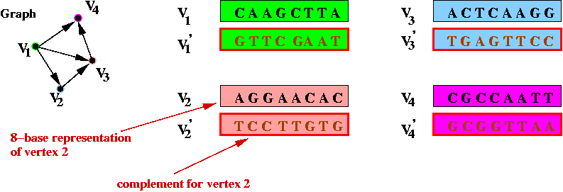
Step 1 (on paper): associate unique DNA substrings with vertices, e.g.
- In the above example, an 8-base string represents a vertex.
- In practice, a larger number is required to help separate out different-length paths.
Step 2 (on paper): associate unique DNA substrings with edges, based on substrings for vertices:
- For edge ( v₁, v₂) join the latter half of v₁'s string with the first half of v₂'s string.
Step 3 (on paper): identify the complementary strings for the vertices, e.g.,
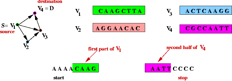
Step 4 (on paper): create unique "start" and "stop" DNA strings for vertices s and d.
- The "start" string represents an artifical edge between "start" and s.
- The "end" string represents an artifical edge between d and "end".
Step 5 (lab): synthesize all of the above DNA material (substrings) separately (one beaker corresponding to each different string).
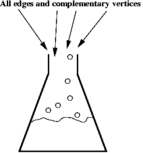
Step 6 (lab): mix all the edges and complementary vertices:
- The complementary vertices will, lego-like, bind edges in sequence.
- This will produce all possible paths in the graph, including invalid ones (without "start" and "end").
  Exercise: Why does this produce all paths?
Step 6 (lab): extract all paths beginning with "start" and ending with "end".
=> use PCR techniques
Step 7 (lab): separate out the DNA with the correct length (exactly n substrings)
=> use gel-electrophoresis.
- Note: this will result in paths of exactly length n.
- However, it will also contain paths with repetitions.
Step 8 (lab):
- Filter out all paths that don't contain the string for v₁
  => use v'₁ (complement) to bind.
- This leaves all paths containing v₁.
- Next, filter out all paths that don't contain v₂.
- ... (repeat for all vertices)
- What remains: the DNA representation of all paths of length n that contain all vertices
  => Hamiltonian paths!

Summary:

The purpose was to show that DNA and chemical processes can "compute".
Potential efficiency: chemical reactions occur in parallel.
It is not yet a practical method:
- Problems need to be carefully coded.
- Encoding takes time.
- Macro-scale experimentation results in errors
  => (fraction of a teaspoonful required for 7-vertex graph).
Related work:
- Using DNA for building "wetware" (gates, flip-flops).
- Using proteins for computation.
- Self-assembling nanotechnology.

Genetic Algorithms and Combinatorial Optimization Problems

Key ideas:

Use evolution as a metaphor for "winnowing" solutions.

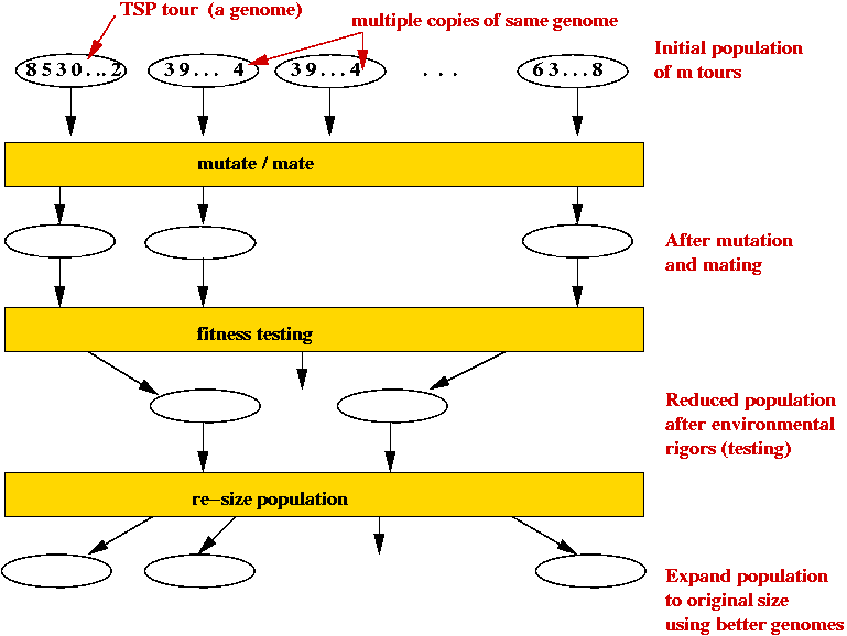
Outline (for TSP):

Each candidate TSP tour is a "genome" (animal).
Start with a large number of potential solutions (initial population).
At each step generate a new population:
- Use mutation to "explore"
- Use mating to preserve "good characteristics".
Weak (high-cost) solutions "die".
Strong (low-cost) solutions "survive".
Eventually, optimal solution should dominate population.

Details: (TSP example)

Input: the n TSP points.
Associate tour with genome.
A genome's fitness is the tour's length.
(shorter the better).
Step 1: create an initial population of m random tours (.e.g, m = 1000).
(They don't have to be unique).

Step 2: Compute the "fitness" value of each genome (tour).
Example with four 5-city tours:

ID	Genome (tour)	Fitness (inverse tour length)	Fraction of total (PDF)
1	0-1-2-3-4	27.5	0.31
2	4-0-1-3-2	12.95	0.15
3	0-2-1-3-4	9.3	0.11
4	2-4-3-0-1	36.0	0.42
		87.75 (total)	1.00 (total)

Step 3: compute the population PDF (Probability Distribution Function) => fraction based on fitness.
- Compute the total fitness (sum of tour costs).
- Compute what fraction of the total each fitness value amounts to.
- The fractions are the PDF.
Step 4: generate a new population drawing from the PDF
=> about 31% (on average) of the new population will contain genome 1 and 11% will contain genome 3.
Step 5: Apply crossover rules (mating):
- The crossover-fraction is an algorithm parameter, e.g., crossover-fraction = 0.3
  => 30% of genome-pairs will engage in crossover.
- Select a random 30% of pairs randomly (assuming crossover-fraction = 30).
- Apply a crossover rule to each such pair: exchange parts of genomes between the pair.
Step 6: Apply mutation
- mutation-fraction is an algorithm parameter.
- mutation-fraction = fraction of genomes to mutate
  (e.g., 0.05)
- Select 5% of the genomes (randomly) to mutate.
- Apply mutation to each (make a slight adjustment in the tour).
Repeat steps 2-6 until fitness values converge
=> population is dominated by high-fitness genomes (tours).

Crossover and mutation in TSP:

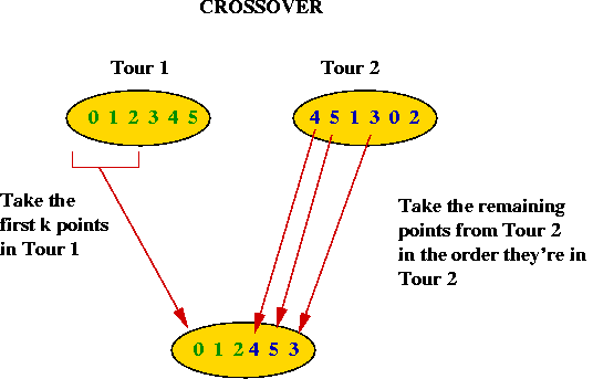
How do we "mate" two TSP tours?
- Take the first part (about half) of Tour 1.
- Take the remaining points in the order these points are found in Tour 2.
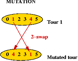
How do we mutate a TSP tour?
=> swap 2 points

Summary:

Advantages of genetic algorithms:
- Genetic algorithms are easy to implement.
- Like simulated annealing, the problem-specific part can be separated out from the generic algorithm.
- If re-arrangements in fact do impact the solution, genetic algorithms have a reasonable chance of finding a good solution.
- By its nature genetic algorithms try many initial solutions (simultaneously)
  => simulated annealing needs to be re-run with different starting solutions.
Disadvantages:
- Genetic algorithms are slow.
- It's hard to define meaningful crossovers and mutations for some problems.
- It requires some experimentation to get it working.
  => it's easier to automate this part in simulated annealing.
- Generally, simulated annealing (with appropriate modification) is thought to be a better option.
Warning:
- Its biological origins do not give it any special advantage
  => beware of its mystical appeal!

Neural Networks

Simplified neuron architecture:

Artificial neuron:

Structure:

Rule: Neuron fires if X₁ + X₂ + X₃ > T.

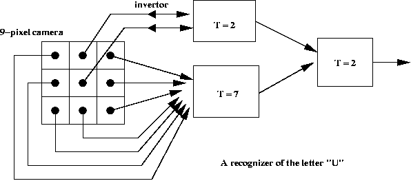
A simple application to pattern recognition:

McCulloch-Pitt neuron model:

Structure:
Inputs: X₁, X₂, ..., X_n
An "importance" weight W_i is associated with each input i.
Neuron has output only if W₁X₁ + ... + W_nX_n > T.

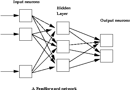
Networks of neurons:

Neural networks are used to approximate unknown functions.
Key ideas:
- Each network has a set of parameters (neuron weights).
- Use a "training set" of samples from unknown function to set parameters.
- Once parameters are set, the function is approximated.