Module 9: Shortest Paths and Dynamic Programming
Single-Source Shortest Paths: Additional Topics
We will now consider three variations of the single-source
shortest-path problem:
- When edges have negative weights.
- Directed graphs.
- DAG's.
Negative weights:
- Some applications require some edges to have negative weights.
- Dijkstra's algorithm does not work with negative weights:
- Recall: once we extract a vertex v from the priority queue,
it is never visited again.
=> if a negative-edge path to v is explored later,
the algorithm does not record it.
- Even adding a large positive number to all edge weights (to
make them positive) does not work. (Why?)
- Negative weight cycles:

- On the left, the path from A to C is not affected by the
positive weight cycle BDE.
- On the right, repeated traversals through BDE keep decreasing
the path length from A to C
=> no solution possible.
- Use the Bellman-Ford Algorithm for negative weights (see
Cormen book):
- Variation of Dijkstra's algorithm.
- Takes O(VE) time.
Directed graphs:
- Dijkstra's algorithm works (almost) without modification for
directed graphs.
- In exploring edges, we must ensure we are only exploring
out-going edges:
- If the graph representation is standard, this is already taken
care of:
- Adjacency-matrix: non-zero entry indicates directed edge.
- Adjacency-list: only out-going edges are in a vertex list.
DAG's:
- DAG's have additional structure (no cycles)
=> is a faster algorithm possible?
- Recall: topological sort takes O(E) time.
- Recall: in Dijkstra's algorithm, vertices are explored in
"priority" order.
- Note:
- In a DAG, exploring a "downstream" vertex cannot affect the
shortest path to an upstream vertex.
- If the source is "downstream", no path is possible.
- Key observation: exploring vertices in topological-sort
order is sufficient.
- Pseudocode:
Algorithm: DAG-SPT (G, s)
Input: Graph G=(V,E) with edge weights and designated source vertex s.

     // Initialize priorities and create empty SPT.
1.   Set priority[i] = infinity for each vertex ;
     // Sort vertices in topological order and place in list.
2.   vertexList = topological sort of vertices in G;
     // Place source in shortest path tree.
3.   priority[s] = 0
4.   Add s to SPT;

     // Process remaining vertices.
5.   while vertexList.notEmpty()
         // Extract next vertex in topological order.
6.       v = extract next vertex in vertexList;
         // Explore edges from v.
7.       for each neighbor u of v
8.           w = weight of edge (v, u);
             // If there's a better way to get to u (via v), then update.
9.           if priority[u] > priority[v] + w
10.              priority[u] = priority[v] + w
11.              predecessor[u] = v
12.          endif
13.      endfor
14.  endwhile

15.  Build SPT;
16.  return SPT

Output: Shortest Path Tree (SPT) rooted at s.
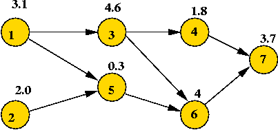
- Vertex-weighted DAG's:
- Consider the case where vertices have weights, but the
edges don't, e.g.,

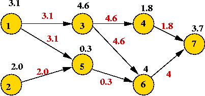
- To find shortest paths, apply a vertex's weight to each
outgoing edge:

- Then solve as a regular DAG-SPT problem.
- Longest path in a vertex-weighted DAG:
- Application: vertices are tasks, weights are time-requirements.
- Objective: find the earliest completion time for the whole
set of tasks.
=> find the longest path.
- Solution:
- Transform into "task DAG" by adding source and sink vertices:

- For each vertex, apply the vertex weight to each outgoing edge.

- Use weight 0 on the source edges.
- Use the "mirror image" (i.e., prefer larger weights)
of the DAG-SPT algorithm above using the newly-added "source"
as s.
Algorithm: maxWeightPath (G, s)
Input: Graph G=(V,E) with edge weights and designated source vertex s.

     // ... initialization same as DAG-SPT ...

5.   while vertexList.notEmpty()
           // ... same as DAG-SPT ...

           // Notice the reversal from ">" to "<":
9.         if priority[u] < priority[v] + w
10.            priority[u] = priority[v] + w
               // ...
12.        endif
14.  endwhile

     // ... same as DAG-SPT ...
Output: Longest Path from source s.
- The longest path is sometimes called the critical
path in a task-graph.
All-Pairs Shortest Paths
The shortest-path between every pair of vertices:
Key ideas in the Floyd-Warshall algorithm:
- Assume the n vertices are numbered 0, ..., n-1
- Let Sk = { vertices 0, ..., k }.
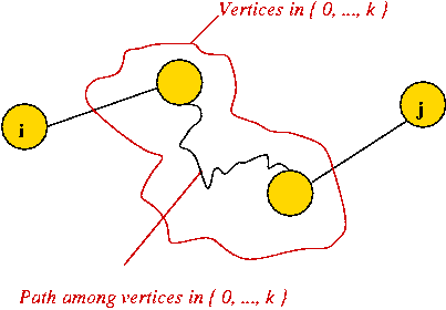
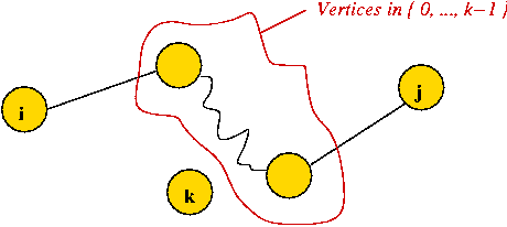
- Consider intermediate vertices on a path between i and j.
- Suppose we force ourselves to use intermediate vertices
only from the set Sk = { 0, 1, 2, ..., k }.

- Note: i and j need not be in Sk.
- It is possible that no such path exists
=> path weight will be infinity.
- Let Dijk = weight of shortest path from i
to j using intermediate vertices in Sk.
- Let wij = weight of edge ij.
- We will let k = -1 define a "base case":
- Because k = -1, no intermediate vertices may be used.
=> Dij-1 = wij,
if an edge from i to j exists.
- If we set wij = infinity when no edge is
present,
=> Dij-1 = wij always.
- Note:
- Dijk-1 = weight of shortest path from i
to j using intermediate vertices in Sk-1 = { 0, 1, 2, ..., k-1 }.
- Now, consider three cases:
- Case 1: k = -1
- Case 2: k >= 0 and vertex k is not in the
Dijk
path from i to j.
- Case 3: k >= 0 and vertex k is in the
Dijk
path from i to j.
- Case 1: k = -1. Here, Dij-1 = wij (from before).
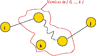
- Case 2: vertex k is not in the path:

- In this case, the intermediate vertices are in Sk-1.

- Thus,
Dijk = Dijk-1.
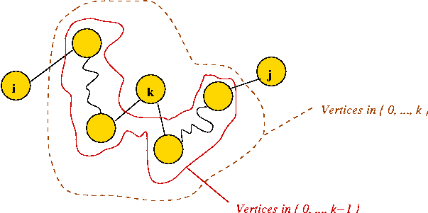
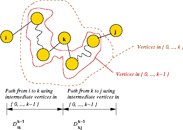
- Case 3: vertex k is in the path:
- Consider the sub-paths not including k:

- By the containment property:

- The path from i to k is the shortest path
from i to k that uses intermediate vertices in Sk-1.
- The path from k to j is the shortest path
from k to j that uses intermediate vertices in Sk-1.
- Thus,
Dijk =
Dikk-1 + Dkjk-1.
- Since only these three cases are possible, one of them must
be true.
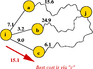
=> when k >= 0, Dijk must be the lesser of
the two values Dijk-1 and
Dikk-1 +
Dkjk-1.
(Otherwise Dijk wouldn't be optimal).
- Thus, combining the three cases:
| Dijk |
= |
wij
min ( Dijk-1,
Dikk-1 +
Dkjk-1 )
|
|
if k = -1
if k >= 0
|
Note:
- The above equation is only an assertion of a property (it's
not an algorithm).
- The equation really says "optimality for size k" can be
expressed in terms of "optimality for size k-1".
- Recall Dijk = optimal cost of going
from i to j using vertices in Sk.
=> the overall optimal cost of going from i to
j is:
Dijn-1 (for n vertices).
- Thus, we need to compute Dijn-1.
- But, this only gives the optimal cost (or weight)
=> we will address the problem of actually identifying the
paths later.
Implementation:
- At first, a recursive approach seems obvious.
- We will use an iterative approach:
- First, compute Dijk for
k=0
(i.e., Dij0)
- Then, use that to compute Dij1.
- ...
- Finally, use Dijn-2 to
compute Dijn-1.
- Pseudocode:
Algorithm: floydWarshall (adjMatrix)
Input: Adjacency matrix representation: adjMatrix[i][j] = weight of
       edge (i,j), if an edge exists; adjMatrix[i][j]=0 otherwise.

      // Initialize the "base case" corresponding to k == -1.
      // Note: we set the value to "infinity" when no edge exists.
      // If we didn't, we would have to include a test in the main loop below.
1.    for each i, j
2.        if adjMatrix[i][j] > 0
3.            Dk-1[i][j] = adjMatrix[i][j]
4.        else
5.            Dk-1[i][j] = infinity
6.        endif
7.    endfor

      // Start iterating over k. At each step, use the previously computed matrix.
8.    for k=0 to numVertices-1

          // Compute Dk[i][j] for each i,j.
9.        for i=0 to numVertices-1
10.           for j=0 to numVertices-1
11.               if i != j
                  // Use the relation between Dk and Dk-1
12.                   if Dk-1[i][j] < Dk-1[i][k] + Dk-1[k][j]     // CASE 2
13.                       Dk[i][j] = Dk-1[i][j]
14.                   else
15.                       Dk[i][j] = Dk-1[i][k] + Dk-1[k][j]      // CASE 3
16.                   endif
17.               endif
18.           endfor
19.       endfor

        // Matrix copy: current Dk becomes next iteration's Dk-1
20.     Dk-1 = Dk

21.   endfor

      // The Dk matrix only provides optimal costs. The
      // paths still have to be built using Dk.
22.   Build paths;
23.   return paths

Output: paths[i][j] = the shortest path from i to j.
- Sample Java code
(source file)
  public void allPairsShortestPaths (double[][] adjMatrix)
  {

    // Dk_minus_one = weights when k = -1
    for (int i=0; i < numVertices; i++) {
      for (int j=0; j < numVertices; j++) {
        if (adjMatrix[i][j] > 0)
          Dk_minus_one[i][j] = adjMatrix[i][j];
        else
          Dk_minus_one[i][j] = Double.MAX_VALUE;
        // NOTE: we have set the value to infinity and will exploit
        // this to avoid a comparison.
      }
    }


    // Now iterate over k.

    for (int k=0; k < numVertices; k++) {

      // Compute Dk[i][j], for each i,j

      for (int i=0; i < numVertices; i++) {
        for (int j=0; j < numVertices; j++) {
          if (i != j) {

            // D_k[i][j] = min ( D_k-1[i][j], D_k-1[i][k] + D_k-1[k][j].
            if (Dk_minus_one[i][j] < Dk_minus_one[i][k] + Dk_minus_one[k][j])
              Dk[i][j] = Dk_minus_one[i][j];
            else
              Dk[i][j] = Dk_minus_one[i][k] + Dk_minus_one[k][j];

          }
        }
      }

      // Now store current Dk into D_k-1
      for (int i=0; i < numVertices; i++) {
        for (int j=0; j < numVertices; j++) {
          Dk_minus_one[i][j] = Dk[i][j];
        }
      }

    } // end-outermost-for


    // Next, build the paths by doing this once for each source.

    // ... (not shown) ...

  }
Analysis:
- The triple for-loop says it all: O(V3).
In-Class Exercise 9.1:
Start with the following template and:
- Write a recursive version of the Floyd-Warshall algorithm.
- Draw the test-case graph on paper and verify that the algorithm
is producing the correct results.
- Count the number of times the recursive function is called
(the main method has a test case).
- In FloydWarshall.java (the sample code above), count the number of times
the innermost if-statement is executed.
- Explain the difference in the two counts.
An optimization:
- Consider Dikk-1
- Dikk-1 = optimal cost from
i to k using Sk.
- Observe: k cannot be an intermediate vertex in an optimal
path that ends at k
=> cost does not change if we allow k to be an intermediate vertex.
=> Dikk-1 = Dikk.
- Similarly,
Dkjk-1 = Dkjk.
- Thus, whether we use Dikk-1
or Dikk makes no difference.
=> we can use the updated matrix
Dikk in loop.
=> only one matrix is needed!
- One more observation: at the time of computing
Dijk, the current "best value" is
Dijk-1.
- Thus, in the pseudocode, we can replace
12.           if Dk-1[i][j] < Dk-1[i][k] + Dk-1[k][j]
13.               Dk[i][j] = Dk-1[i][j]
14.           else
15.               Dk[i][j] = Dk-1[i][k] + Dk-1[k][j]
16.           endif
with
              // The first Dk[i][j] is really Dk-1[i][j]
              // because we haven't written into it yet.
12.           if Dk[i][j] < Dk[i][k] + Dk[k][j]
                  // This is superfluous:
13.               Dk[i][j] = Dk[i][j]
14.           else
                  // This is all we need:
15.               Dk[i][j] = Dk[i][k] + Dk[k][j]
16.           endif
- We will now use a single matrix D[i][j]:
Algorithm: floydWarshallOpt (adjMatrix)
Input: Adjacency matrix representation: adjMatrix[i][j] = weight of
       edge (i,j), if an edge exists; adjMatrix[i][j]=0 otherwise.

      // ... initialization similar to that in floydWarshall ...

1.    for k=0 to numVertices-1

2.        for i=0 to numVertices-1
3.            for j=0 to numVertices-1
4.                if i != j
                      // Use the same matrix.
5.                    if D[i][k] + D[k][j] < D[i][j]
6.                        D[i][j] = D[i][k] + D[k][j]
7.                    endif
8.                endif
9.            endfor
10.       endfor

11.   endfor

      // ... path construction ...
Distributed Routing in a Network
First, consider an iterative version of Floyd-Warshall:
- Consider the following version of the Floyd-Warshall algorithm:
(source file)
Algorithm: floydWarshallIterative (adjMatrix)
Input: Adjacency matrix representation: adjMatrix[i][j] = weight of
       edge (i,j), if an edge exists; adjMatrix[i][j]=0 otherwise.

      // ... initialization similar to that in floydWarshallOpt ...

1.    changeOccurred = true
2.    while changeOccurred

          changeOccurred = false

3.        for i=0 to numVertices-1
4.            for j=0 to numVertices-1
5.                if i != j
                      // "k" is now in the innermost loop.
6.                    for k=0 to numVertices
7.                        if D[i][k] + D[k][j] < D[i][j]
                              // Improved shortest-cost.
8.                            D[i][j] = D[i][k] + D[k][j]
                              // Since this may propagate, we have to continue iteration.
9.                            changeOccurred = true
10.                       endif
11.                   endfor
10.               endif
11.           endfor
12.       endfor

13.   endwhile
      // ... path construction ...
- Why does this work?
- First, examine the original triple for-loop:
    for k=0 to numVertices-1
      for i=0 to numVertices-1
        for j=0 to numVertices-1

        // ... compute with D[i][j], D[i][k] and D[k][j] ...

        endfor
      endfor
    endfor
- Next, suppose we move the outermost for-loop inside:
    for i=0 to numVertices-1
      for j=0 to numVertices-1
        for k=0 to numVertices-1

        // ... compute with D[i][j], D[i][k] and D[k][j] ...

        endfor
      endfor
    endfor
In this case:
- Consider a particular i and j, e.g., 3 and 7.
- Once D[3][7] is computed, we never return to it again.
- Suppose D[4][5] (computed later) affects D[3][7]
=> we won't modify D[3][7] (as we should).
- On the other hand, if no other D[i][j] changes, then
D[3][7] is correctly computed.
- If we keep track of whether something changed, it works.
- This does not seem more efficient (it is not), but it's
a useful observation for distributed routing.
What do we mean by "distributed routing"?
- A "network" is a collection of computers connected together in
some fashion (with links)
=> can represent a network using a graph.
- Example: internet routers connected by links.
- A "routing algorithm" provides for data to get sent across
the network.
- Centralized vs. Distributed:
- Routes can be computed centrally by a server.
- Or in a distributed fashion by routers (since routers are
also, typically, computers).
- Routes are computed frequently (e.g., as often as 30 milliseconds)
=> need an efficient way to computed routes.
In-Class Exercise 9.2:
Why aren't routes computed just once and for all whenever a network is
initialized?
Distributed Floyd-Warshall: a purely distibuted algorithm
- Consider the iterative version:
    while changeOccurred

        for i=0 to numVertices-1
            for j=0 to numVertices-1

            // Node i says "let me try to get to destination j via k".
            for k=0 to numVertices
                // If it's cheaper for me to go via k, let me record that.
                if D[i][k] + D[k][j] < D[i][j]
                    // Improved shortest-cost: my cost to neighbor k, plus k's cost to j
                    D[i][j] = D[i][k] + D[k][j]
                    changeOccurred = true
                endif

            endfor
         endfor

   endwhile
- Key ideas:
- Each node maintains its current shortest-cost to each destination.
- Thus, node i maintains the value
Di[j] = "current best cost to get to destination j".
- Node i polls its neighbors asking them "how much does
it cost you to get to j?".

- Node i uses these replies (and its own costs to get to
neighbors) to find the best path.
- This process is repeated as long as changes propagate.
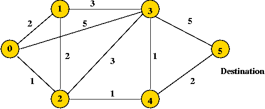
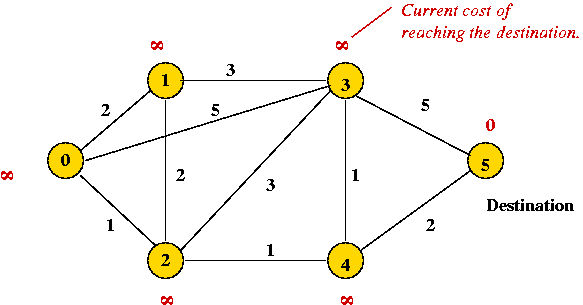
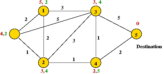
- Example:

- We will show computations when node "5" is the destination.
=> in practice, the computation for all destinations
occurs simultaneously.
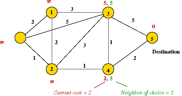
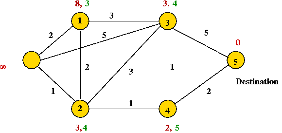
- Each node maintains:
- Its currently-known cost to get to "5",
- Which neighbor is used in getting to "5"
Initially, nothing is known:

- After the first round of message-exchange between neighbors:

- After the next round:

- After the next round:

- The next round reveals no changes
=> algorithm halts (nodes stop exchanging information).
A semi-distributed algorithm: running Dijkstra at each node
- All nodes acquire complete information about the network
=> topology and edge weights.
- Each node runs Dijkstra's algorithm with itself as root.
=> each node know which outgoing link to use to send data (to
a particular destination).
- How is edge-information exchanged?
- Use a broadcast or flooding algorithm (separate topic).
The process of "routing":
- How is a packet of data routed?
- Each node maintains a routing table
e.g., the table at node 0 in the earlier example
| Destination | Current cost | Outgoing link |
| ... | ... | ... |
| ... | ... | ... |
| 5 | 4 | (0,2) |
| ... | ... | ... |
- When a packet comes in, the destination written in the
packet is "looked up" in the table to find the next link.
- Destination-based routing:
- The routing table is indexed only by destination.
- This is because of the "containment" property of
shortest-path routing.
- Example: (above) whenever a packet for 5 comes into node 0, it
always goes out on link (0, 2).
=> it doesn't matter where the packet came from.
- Destination-based routing is simpler to implement.
- Alternative: routing based on both source and destination.
=> requires more space.
| Source | Destination | Current cost | Outgoing link |
| ... | ... | ... | ... |
| ... | ... | ... | ... |
| 1 | 5 | x | (0,2) |
| ... | ... | ... | ... |
| 0 | 5 | y | (0,3) |
| ... | ... | ... | ... |
Internet routing:
- The old internet (up to mid-80's) used a version of distributed-Floyd-Warshall.
=> called RIP (Routing Information Protocol).
- RIP has problems with looping.
=> mostly discontinued (but still used in places).
- The current protocol (called OSPF) uses the semi-distributed
Dijkstra's algorithm described above.
- We have only discussed the important algorithmic ideas
=> many more issues in routing (link failures,
control-messages, loop-prevention etc).
Dynamic Programming (Contiguous Load Balancing Example)
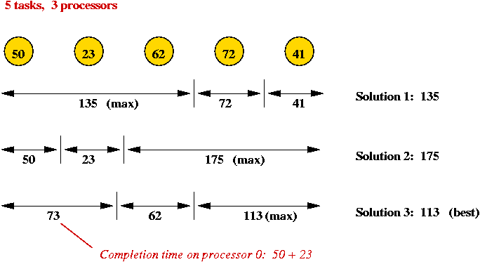
Consider the following problem: (Contiguous Load Balancing)
- Input:
- A collection of n tasks.
- Task i takes si time to complete.
- A collection of m processors.
- Goal: assign tasks to processors to minimize completion time.
- Note:
- Each processor must be assigned a contiguous subset of tasks
(e.g., the tasks i, ..., i+k).
- The completion time for a processor is the sum of task-times
for the tasks assigned to it.
- The overall completion time for the system is the maximum
completion time among the processors.
- Example:

In-Class Exercise 9.3:
Write an algorithm to take as input (1) the task times, and (2) the
number of processors, and produce a (contiguous) partition of tasks
among the processors. Start by downloading
this template.
What is dynamic programming?
- First, the key ideas have very little to do with "dynamic" and
"programming" as we typically understand the terms.
(The terms have a historical basis).
- "Dynamic programming" is an optimization technique
=> applies to some optimization problems.
- OK, what is an optimization problem?
- Usually, a problem with many candidate solutions.
- Each candidate solution results in a "value" or "cost".
- Goal: find the solution that minimizes cost (or maximizes value).
- Example: in the load balancing problem, we want to
minimize the overall completion time.
- It's initially hard to understand and, sometimes, apply.
But it's very effective when it works.
- To gauge whether a problem may be suitable for dynamic
programming:
- The problem should divide easily into sub-problems.
- It should be possible to express the optimal value for the
problem in terms of the optimal value of sub-problems.
- General procedure:
- Initially ignore the actual solution and instead examine only the "value".
- Find a relation between the optimal value for
problem of size i and that of size i-1.
(If there are two or more parameters, the recurrence is
more complicated).
- Write the relation as a recurrence.
- Write down base cases.
- Solve iteratively (most often) or recursively, depending on the problem.
- Write additional code to extract the candidate solutions as
the dynamic programming progresses
(or even afterwards, as we did with shortest paths).
Example: dynamic programming applied to the load balancing problem
- Let Dik = optimal cost for
tasks 0, ..., i and k processors.
- Note: this problem has two parameters: i and k.
- The "dynamic programming" relation:
Dik
= minj max { Djk-1,
sj+1 + ... + si }
(where j ranges over { 0, ..., i }).
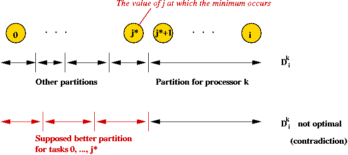
- Why is this true?

- Suppose that in the optimal solution, partition k-1
ends at task j*.
- This means that tasks (j* + 1), ..., i are in the last partition.
- If there's a better partition of 0, ..., j*, it would
be used in the optimal solution!
- General principle: the optimal solution for i is
expressed in terms of the optimal solutions to smaller problems.
(because the solution to smaller problems is independent).
- In this case:
Optimal solution to
problem of size (k, i) |
= |
Combination of
(maximum of) |
optimal solution to
problem of size (k-1, j)
(for some j) |
and |
some computation
(sum across last partition) |
In terms of the equation:
|
Dik
|
= |
max |
(Dj*k-1,
|
sj*+1 + ... + si)
|
- We still require some searching: we try each sub-problem
of size (k-1, j).
- Base cases:
- What are the possible values of i and k?
- Input to problem: tasks 0, ..., n-1 and m processors.
- Thus, by the definition of Dik:
- i ranges from 0 to n-1
- k ranges from 1 to m.
- Base cases: Di1
= s0 + ... + si (for each i).
(only one processor)
Implementation:
- Note: to use "optimal values" of sub-problems, we need to
either store them or compute recursively.
- Since sub-problems reappear, it's best to store them.
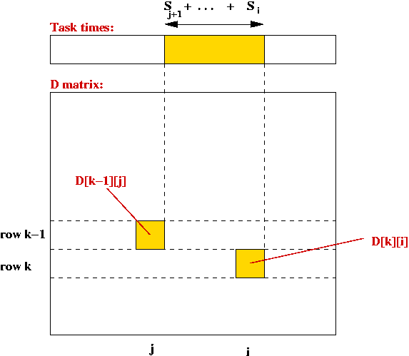
- We will use a matrix D[k][i] to store Dik.
- Pseudocode:
Algorithm: dynamicProgrammingLoadBalancing (numTasks, taskTimes, numProcessors)
Input: the number of tasks (numTasks), the number of processors (numProcessors),
       taskTimes[i] = time required for task i.

      // Initialization. First, the base cases:
1.    D[1][i] = sum of taskTimes[0], ... ,taskTimes[i];
      // We will set the other values to infinity and exploit this fact in the code.
2.    D[k][i] = infinity, for all i and k > 1

      // Now iterate over the number of processors.
3.    for k=2 to numProcessors
          // Optimally allocate i tasks to k processors.
4.        for i=0 to numTasks-1

              // Find the optimal value of D[k][i] using prior computed values.
5.            min = max = infinity
              // Try each value of j in the recurrence relation.
6.            for j=0 to i
                  // Compute sj+1 + ... + si
7.                sum = 0
8.                for m=j+1 to i
9.                    sum = sum + taskTimes[m]
10.               endfor
                  // Use the recurrence relation.
11.               max = maximum (D[k-1][j], sum)
                  // Record the best (over j).
12.               if max < min
13.                   D[k][i] = max
14.                   min = max
15.               endif
16.           endfor // for j=0 ...

          // Optimal D[k][i] found.
17.       endfor // for i=0 ...
18.   endfor // outermost: for k=2 ...

18.   Find the actual partition;
19.   return partition
Output: the optimal partition
- Sample Java code:
(source file)
  static int[] dynamicProgramming (double[] taskTimes, int numProcessors)
  {
    int numTasks = taskTimes.length;

    // If we have enough processors, one processor per task is optimal.
    if (numProcessors >= numTasks) {
      int[] partition = new int [numTasks];
      for (int i=0; i < numTasks; i++)
        partition[i] = i;
      return partition;
    }

    // Create the space for the array D.
    double[][] D = new double [numProcessors+1][];
    for (int p=0; p<=numProcessors; p++)
      D[p] = new double [numTasks];

    // Base cases:
    for (int i=0; i < numTasks; i++) {
      // Set D[1][i] = s_0 + ... + s_i
      double sum = 0;
      for (int j=0; j<=i; j++)
        sum += taskTimes[j];
      D[1][i] = sum;
      for (int k=i+2; k<=numProcessors; k++)
        D[k][i] = Double.MAX_VALUE;
      // Note: we are using MAX_VALUE in lieu of INFINITY.
    }


    // Dynamic programming: compute D[k][i] for all k
    // Now iterate over the number of processors.
    for (int k=2; k<=numProcessors; k++) {

      // In computing D[k][i], we iterate over i second.
      for (int i=0; i < numTasks; i++) {

        // Find the optimal value of D[k][i] using
        // prior computed values.

        double min = Double.MAX_VALUE;
        double max = Double.MAX_VALUE;

        // Try each value of j in the recurrence relation.
        for (int j=0; j<=i; j++) {

          // Compute sj+1 + ... + si
          double sum = 0;
          for (int m=j+1; m<=i; m++)
            sum += taskTimes[m];

          // Use the recurrence relation.
          max = D[k-1][j];
          if (sum > max) {
            max = sum;
          }

          // Record the best (over j).
          if (max < min) {
            min = max;
            D[k][i] = min;
          }
        } // end-innermost-for

      } // end-second-for

      // Optimal D[k][i] found.

    } //end-outermost-for


    // ... compute the partition itself (not shown) ...
  }
- How to compute the partition?
- Each time the minimal value in the scan (over
j) is found, record the position.
- The first time you do this, you get the last partition.
- This also tells you the D[k-1][j] to use next.
- Work backwards (iteratively) to find the previous partition
... and so on.
- What the matrix looks like at an intermediate stage:

Example:
- 5 tasks, 3 processors.
- Task times:
| Task |
0 |
1 |
2 |
3 |
4 |
| Time |
50 |
23 |
62 |
72 |
41 |
- For this problem successive values of the matrix is
shown with the current value in red
and the D[k-1][j*] value in purple:
k = 2, i = 0
| 0.0 | 0.0 | 0.0 | 0.0 | 0.0 |
| 50.0 | 73.0 | 135.0 | 207.0 | 248.0 |
| 50.0 | 0.0 | 0.0 | 0.0 | 0.0 |
| INF | INF | 0.0 | 0.0 | 0.0 |
k = 2, i = 1
| 0.0 | 0.0 | 0.0 | 0.0 | 0.0 |
| 50.0 | 73.0 | 135.0 | 207.0 | 248.0 |
| 50.0 | 50.0 | 0.0 | 0.0 | 0.0 |
| INF | INF | 0.0 | 0.0 | 0.0 |
k = 2, i = 2
| 0.0 | 0.0 | 0.0 | 0.0 | 0.0 |
| 50.0 | 73.0 | 135.0 | 207.0 | 248.0 |
| 50.0 | 50.0 | 73.0 | 0.0 | 0.0 |
| INF | INF | 0.0 | 0.0 | 0.0 |
k = 2, i = 3
| 0.0 | 0.0 | 0.0 | 0.0 | 0.0 |
| 50.0 | 73.0 | 135.0 | 207.0 | 248.0 |
| 50.0 | 50.0 | 73.0 | 134.0 | 0.0 |
| INF | INF | 0.0 | 0.0 | 0.0 |
k = 2, i = 4
| 0.0 | 0.0 | 0.0 | 0.0 | 0.0 |
| 50.0 | 73.0 | 135.0 | 207.0 | 248.0 |
| 50.0 | 50.0 | 73.0 | 134.0 | 135.0 |
| INF | INF | 0.0 | 0.0 | 0.0 |
k = 3, i = 0
| 0.0 | 0.0 | 0.0 | 0.0 | 0.0 |
| 50.0 | 73.0 | 135.0 | 207.0 | 248.0 |
| 50.0 | 50.0 | 73.0 | 134.0 | 135.0 |
| 50.0 | INF | 0.0 | 0.0 | 0.0 |
k = 3, i = 1
| 0.0 | 0.0 | 0.0 | 0.0 | 0.0 |
| 50.0 | 73.0 | 135.0 | 207.0 | 248.0 |
| 50.0 | 50.0 | 73.0 | 134.0 | 135.0 |
| 50.0 | 50.0 | 0.0 | 0.0 | 0.0 |
k = 3, i = 2
| 0.0 | 0.0 | 0.0 | 0.0 | 0.0 |
| 50.0 | 73.0 | 135.0 | 207.0 | 248.0 |
| 50.0 | 50.0 | 73.0 | 134.0 | 135.0 |
| 50.0 | 50.0 | 62.0 | 0.0 | 0.0 |
k = 3, i = 3
| 0.0 | 0.0 | 0.0 | 0.0 | 0.0 |
| 50.0 | 73.0 | 135.0 | 207.0 | 248.0 |
| 50.0 | 50.0 | 73.0 | 134.0 | 135.0 |
| 50.0 | 50.0 | 62.0 | 73.0 | 0.0 |
k = 3, i = 4
| 0.0 | 0.0 | 0.0 | 0.0 | 0.0 |
| 50.0 | 73.0 | 135.0 | 207.0 | 248.0 |
| 50.0 | 50.0 | 73.0 | 134.0 | 135.0 |
| 50.0 | 50.0 | 62.0 | 73.0 | 113.0 |
Analysis:
- Assume: n tasks, m processors.
- The three inner for-loops each range over tasks:
=> O(n3).
- The outermost for-loop ranges over processors
=> O(m n3) overall.
- We have used a m x n array
=> O(m n) space.
- Reducing space:
- Since only the previous row is required, we can manage with
O(n) space (for two rows).
- However, in reconstructing the partition we will need
O(m n) space.
An optimization:
- The innermost for-loop repeatedly computes sums.
- We can pre-compute partial sums and use differences.
- Pseudocode:
Algorithm: dynamicProgrammingLoadBalancing (numTasks, taskTimes, numProcessors)
Input: the number of tasks (numTasks), the number of processors (numProcessors),
       taskTimes[i] = time required for task i.

      // Precompute partial sums
      for i=0 to numTasks
          partialSum[i] = 0
          for j=0 to i
              partialSum = partialSum + taskTimes[i]
          endfor
      endfor

      // ... Remaining initialization as before ...

      for k=2 to numProcessors
          for i=0 to numTasks-1

              for j=0 to i

                  // Note: sj+1 + ... + si = partialSum[i]-partialSum[j]

                  // Use the recurrence relation.
                  max = maximum (D[k-1][j], partialSum[i] - partialSum[j])

                  // ... remaining code is identical ...
- This reduces the complexity to O(m n2).
Dynamic Programming (Floyd-Warshall Algorithm)
The Floyd-Warshall Algorithm used earlier is actually dynamic
programming:
- Recall:
- Let Sk = { vertices 0, ..., k }.
- Let Dijk = weight of shortest path from i
to j using intermediate vertices in Sk.
- The recurrence relation:
| Dijk |
= |
wij
min ( Dijk-1,
Dikk-1 +
Dkjk-1 )
|
|
if k = -1
if k >= 0
|
- Observe:
- This recurrence uses three parameters: i, j and k.
- The optimal value for the larger problem
(Dijk) is expressed in terms of
the optimal values of smaller sub-problems
(Dijk-1, Dikk-1
and Dkjk-1).
- There are more base cases, and more sub-problems, but the
idea is the same.
- Initially, it appears that O(n3) space is
required (for a 3D array).
- However, only successive k values are needed
=> 2D array is sufficient.
Dynamic Programming (Maximum Subsequence Sum Example)
Consider the following problem:
- Given a sequence of n (possibly negative) numbers
x0 , x1 , ..., xn-1
find the contiguous subsequence
xi , ..., xj
whose sum is the largest.
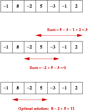
- Example:

- We'll consider the case where the data has at least one
positive number.
=> this can be checked in time O(n).
In-Class Exercise 9.4:
Implement the naive and most straightforward approach: try all possible
contiguous subsequences.
Start by downloading this template.
For now, ignore the template for the faster algorithm.
Using dynamic programming:
- This example will show an unusual use of dynamic programming: how
a different sub-problem is used in the solution.
- We'll start with solving another problem: find the largest
suffix for each prefix.
- The solution to the largest subsequence problem will use this
as a sub-problem.
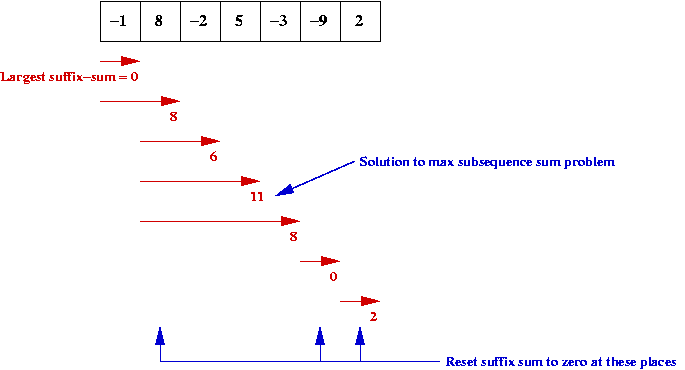
Largest suffix (of a prefix):
- Given numbers
x0 , x1 , ..., xn-1
find, for each k, the largest-sum suffix of the numbers
x0 , x1 , ..., xk
where the sum is taken to be zero, if negative.
- Example:

Dynamic programming algorithm for suffix problem:
Dynamic programming algorithm for subsequence problem:
- Note: the largest subsequence-sum is one of the suffix solutions.
- Hence, all we have to do is track the largest one.
- Define Sk as the maximum subsequence-sum
for the elements
x0 , x1 , ..., xk
- Then, Sk is the best suffix-sum seen so far:
| Sk |
= |
Dk-1 + xk
Sk-1
|
|
if Dk-1 + xk > Sk-1
otherwise
|
- Note: we don't need to store previous values
=> can use a single variable
- Thus, in pseudocode:
Algorithm: maxSubsequenceSum (X)
Input: an array of numbers, at least one of which is positive

      // Initial value of D
  1.  if X[0] > 0
  2.      D = X[0]
  3.  else
  4.      D = 0
  5.  endif

      // Initial value of S, the current best max
  6.  S = X[0]

      // Single scan
  7.  for k = 1 to n-1
          // Update S
  8.      if D + X[k] > S
  9.          S = D + X[k]
  10.     endif
          // Update D
  11.     if D + X[k] > 0
  12.         D = D + X[k]
  13.     else
  14    .     D = 0
  15.     endif
  16. endfor

  17. return S
- Time taken: O(n)
- What's unusual about this problem:
- Unlike the other problems in this section, the decomposition
tracked the partial solutions of two problems.
- The dynamic programming equation for subsequence
used the suffix-problem.
In-Class Exercise 9.5:
Implement the faster algorithm and compare with the naive algorithm.
Dynamic Programming (Optimal Binary Tree Example)
Consider the following problem:
- We are given a list of keys that will be repeatedly accessed.
- Example: The keys "A", "B", "C", "D" and "E".
- An example access pattern: "A A C E D B C E A A A A E D D D" (etc).
- We are also given access frequencies (probabilities) , e.g.
| Key | Access probability |
| A | 0.4 |
| B | 0.1 |
| C | 0.2 |
| D | 0.1 |
| E | 0.2 |
(Thus, "A" is most frequently accessed).
- Objective: design a data structure to enable accesses as
rapidly as possible.
Past solutions we have seen:
- Place keys in a balanced binary tree.
=> a frequently-accessed item could end up at a leaf.
- Place keys in a linked list (in decreasing order of probability).
=> lists can be long, might required O(n) access time
(even on average).
- Use a self-adjusting data structure (list or self-adjusting tree).
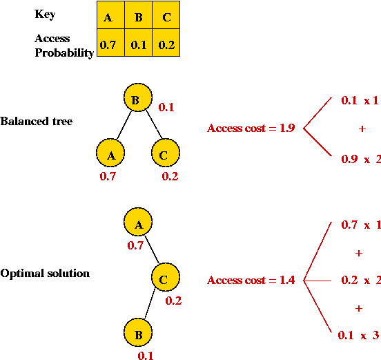
Optimal binary search tree:
- Analogue of the optimally-arranged list.
- Idea: build a binary search tree (not necessarily balanced)
given the access probabilities.
- Example:

- Overall objective: minimize average access cost:
- For each key i, let d(i) be its depth in the
tree
(Root has depth 1).
- Let pi be the probability of access.
- Assume n keys.
- Then, average access cost = d(0)*p0 + ... + d(n-1)*pn-1.
Dynamic programming solution:
- First, sort the keys.
(This is easy and so, for the remainder, we'll assume keys
are in sorted order).
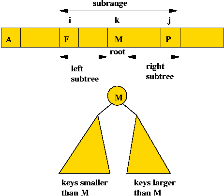
- Suppose keys are in sorted order:
- If we pick the k-th key to be the root.
=> keys to the left will lie in the left sub-tree and keys
to the right will lie in the right sub-tree.
- This also works for any sub-range i, ..., j of the keys:

- Define C(i,j) = cost of an optimal tree formed using
keys i, ..., j (both inclusive).
- Now suppose, in the optimal tree, the root is "the key at
position k".
- The left subtree has keys in the range i, ..., k-1.
=> optimal cost of left subtree is C(i, k-1).
- The right subtree has keys k+1, ..., j.
=> optimal cost of right subtree is C(k+1, j).
- It is tempting to assume that C(i, j) = C(i, k-1) +
C(k+1, j)
=> this doesn't account for the additional depth of the left
and right subtrees.
- The correct relation is:
C(i, j) = pk + C(i, k-1) + (pi +
... + pk-1) + C(k+1, j) + (pk+1 + ... + pj).
- Here, we have added 1 to the depth of each element in the
subtrees.
=> to account for it, we include each probability once again.
- More compactly:
C(i, j) = C(i, k-1) + C(k+1, j) + (pi + ... + pj).
- Now, we assumed the optimal root for C(i, j) was the k-th key.
=> in practice, we must search for it.
=> consider all possible keys in the range i, ..., j
as root.
- Hence the dynamic programming recurrence is:
C(i, j) = mink C(i, k-1) + C(k+1, j) + (pi + ... + pj).
(where k ranges over i, ..., j).
- The solution to the overall problem is: C(0, n-1).
- Observe:
- Once again, we have expressed the cost of the
optimal solution in terms of the optimal cost of sub-problems.
- Base case: C(i, i) = pi.
Implementation:
- Writing code for this case is not as straightforward as in
other examples:
- In other examples (e.g., load balancing), there was a natural
sequence in which to "lay out the sub-problems".
- Consider the following pseudocode:
    // Initialize C and apply base cases.
    for i=0 to numKeys-2
        for j=i+1 to numKeys-1
            min = infinity
            sum = pi + ... + pj;
            for k=i to j
                if C(i, k-1) + C(k+1, j) + sum < min
                    min = C(i, k-1) + C(k+1, j) + sum
          ...
Suppose, above, i=0, j=10 and k=1 in the innermost loop
- The case C(i, k-1) = C(0,0) is a base case.
- But the case C(k+1, j) = C(2, 10) has NOT been
computed yet.
- We need a way to organize the computation so that:
- Sub-problems are computed when needed.
- Sub-problems are not re-computed unnecessarily.
- Solution using recursion:
- Key idea: use recursion, but check whether computation has
occurred before.
- Pseudocode:
Algorithm: optimalBinarySearchTree (keys, probs)
Input: keys[i] = i-th key,  probs[i] = access probability for i=th key.

      // Initialize array C, assuming real costs are positive (or zero).
      // We will exploit this entry to check whether a cost has been computed.
1.    for each i,j set C[i][j] = -1;
      // Base cases:
2.    for each i, C[i][i] = probs[i];

      // Search across various i, j ranges.
3.    for i=0 to numKeys-2
4.        for j=i+1 to numKeys-1
              // Recursive method computeC actually implements the recurrence.
5.            C[i][j] = computeC (i, j, probs)
6.        endfor
7.    endfor

      // At this point, the optimal solution is C(0, numKeys-1)
8.    Build tree;
9.    return tree

Output: optimal binary search tree
Algorithm: computeC (i, j, probs)
Input: range limits i and j, access probabilities

     // Check whether sub-problem has been solved before.
     // If so, return the optimal cost. This is an O(1) computation.
1.   if (C[i][j] >= 0)
2.       return C[i][j]
3.   endif

     // The sum of access probabilities used in the recurrence relation.
4.   sum = probs[i] + ... + probs[j];

     // Now search possible roots of the tree.
5.   min = infinity
6.   for k=i to j
         // Optimal cost of the left subtree (for this value of k).
7.       Cleft = computeC (i, k-1)
         // Optimal cost of the right subtree.
8.       Cright = computeC (k+1, j)
         // Record optimal solution.
9.       if Cleft + Cright < min
10.          min = Cleft + Cright
11.      endif
12.  endfor

13.  return min

Output: the optimal cost of a binary tree for the sub-range keys[i], ..., keys[j].
- In the above pseudocode, we have left out a small detail:
we need to handle the case when a subrange is invalid (e.g., when k-1 < i).
(Can you see how to do it easily?)
Analysis:
- The bulk of the computation is a triple for-loop, each ranging
over n items (worst-case)
=> O(n3) overall.
- Note: we still have account for the recursive calls:
- Each recursive call that did not enter the innermost loop,
takes time O(1).
- But, this occurs only O(n2) times.
=> Overall time is still O(n3).

