Module 7: Graphs, Part I
What is a Graph?
In-Class Exercise 7.0:
Let's start with a simple exercise: The
Calling Circle Problem.
Informal definition:
- A graph is a mathematical abstraction used to represent
"connectivity information".
- A graph consists of vertices and edges that
connect them, e.g.,
- It shouldn't be confused with the "bar-chart" or "curve" type
of graph.
Formally:
- A graph G = (V, E) is:
- a set of vertices V
- and a set of edges E = { (u, v): u and v are vertices }.
- Two types of graphs:
- Undirected graphs: the edges have no direction.
- Directed graphs: the edges have direction.
- Example: undirected graph
- Edges have no direction.
- If an edge connects vertices 1 and 2, either
convention can be used:
- No duplication: only one of (1, 2) or (2, 1)
is allowed in E.
- Full duplication: both (1, 2) and (2, 1)
should be in E.
- Example: directed graph
- Edges have direction (shown by arrows).
- The edge (3, 6) is not the same as the edge (6,
3) (both exist above).
Depicting a graph:
- The picture with circles (vertices) and lines (edges) is
only a depiction
=> a graph is purely a mathematical abstraction.
- Vertex labels:
- Can use letters, numbers or anything else.
- Convention: use integers starting from 0.
=> useful in programming, e.g. degree[i] = degree
of vertex i.
- Edges can be drawn "straight" or "curved".
- The geometry of drawing has no particular meaning:
Graph conventions:
- What's allowed (but unusual) in graphs:
- Self-loops (occasionally used).
- Multiple edges between a pair of vertices (rare).
- Disconnected pieces (frequent in some applications).
Example:
- What's not (conventionally) allowed:
- Mixing undirected and directed edges.
- Re-using labels in vertices.
- Bidirectional arrows.
- Most common:
- No multiple edges.
- No self-loops.
- Other terms used:
- Vertices: nodes, terminals, endpoints.
- Edges: links, arcs.
In-Class Exercise 7.1:
If we disallow multiple edges and self-loops, what is the maximum
number of edges in an undirected graph with n vertices?
What is this number in order-notation?
Definitions:
- Degrees:
- Undirected graph: the degree of a vertex is the
number of edges incident to it.
- Directed graph: the out-degree is the number of (directed) edges
leading out, and the in-degree is the number of
(directed) edges terminating at the vertex.
- Neighbors:
- Two vertices are neighbors (or are adjacent) if
there's an edge between them.
- Two edges are neighbors (or are adjacent) if
they share a vertex as an endpoint.
- Paths:
- Undirected: a sequence of vertices in which successive
vertices are adjacent.
- Directed: a sequence of vertices in which every pair of successive vertices
has this property: there's a directed edge from the first to the second.
- A simple path does not repeat any vertices (and
therefore edges) in the sequence.
- A cycle is a simple path with the same vertex as the
first and last vertex in the sequence.
- Connectivity:
- Undirected: Two vertices are connected if there is a
path that includes them.
- Directed: Two vertices are strongly-connected if there
is a (directed) path from one to the other.
- Components:
- A subgraph is a subset of vertices together with the
edges from the original graph that connects vertices in the subset.
- Undirected: A connected component is a subgraph in
which every pair of vertices is connected.
- Directed: A strongly-connected component is a subgraph
in which every pair of vertices is strongly-connected.
- A maximal component is a connected component that is
not a proper subset of another connected component.
- Digraph: another name for a directed graph.
Example:
More definitions:
Why are graphs important?
- History:
- Applications:
- Fundamental mathematical construct to represent "connectivity".
- Appears in thousands of problems.
- Source of many classic problems: traveling salesman, routing,
spanning trees.
- Many "graph-structured" applications: networks,
transportation-systems, electronic circuits, molecules.
- Source of theory:
- Many important algorithms.
- Key to understanding algorithm design and analysis.
- Simple to describe, yet perplexing:
- Euler tour: easy problem.
- Hamiltonian tour: hard problem.
The field of graph theory:
- Large area of mathematics:
- Analysis of general graphs.
- Analysis of special types of graphs.
- Many classic problems
e.g., the four-color theorem.
- Optimization problems based on graphs,
e.g., shortest-paths.
- Graph algorithms: an area in computer science.
- Rich source of algorithms, theory, insight.
- Useful algorithms used in many applications
(e.g., in a compiler).
In this course:
- Fundamental algorithms for exploring a graph: breadth-first and depth-first.
- Finding shortest paths and minimum spanning tree.
- Convention about undirected vs. directed:
- When not specified, assume undirected.
- Unless otherwise mentioned, an algorithm or definition about
undirected graphs usually can be modified to apply to directed graphs.
(although, directed graphs are usually more complicated).
In-Class Exercise 7.2:
Suppose di is the degree of vertex i in
a connected undirected graph with n vertices and
m edges.
Let D = d1 + ... + dn.
What is the relation between D and m?
Graph Data Structures
First, an idea that doesn't work:
- We have already represented trees (like binary trees) with node
instances and pointers between instances.
- Idea: use a node instance for each vertex, and a pointer from
one vertex to another if an edge exists between them.
In-Class Exercise 7.3:
Why doesn't it work?
The two fundamental data structures:
- Adjacency matrix.
- Key idea: use a 2D matrix.
- Row i has "neighbor" information about vertex i.
- Undirected: adjMatrix[i][j] = 1 if and only if there's an edge
between vertices i and j.
adjMatrix[i][j] = 0 otherwise.
- Directed: adjMatrix[i][j] = 1 if and only if there's an edge
from i to j.
adjMatrix[i][j] = 0 otherwise.
- Example: undirected
      0 1 1 0 0 0 0 0
      1 0 1 0 0 0 0 0
      0 1 0 1 0 1 0 0
      0 0 1 0 1 0 1 0
      0 0 0 1 0 0 1 0
      0 0 1 0 0 0 1 1
      0 0 0 1 1 0 0 0
      0 0 0 0 0 1 0 0
Note: adjMatrix[i][j] == adjMatrix[j][i] (convention for
undirected graphs).
- Example: directed
      0 1 0 0 0 0 0 0
      0 0 1 0 0 0 0 0
      1 0 0 1 0 1 0 0
      0 0 0 0 1 0 1 0
      0 0 0 0 0 0 1 0
      0 0 1 0 0 0 0 1
      0 0 0 1 0 0 0 0
      0 0 0 0 0 0 0 0
- Adjacency list.
- Key idea: use an array of vertex-lists.
- Each vertex list is a list of neighbors.
- Example: undirected
- Example: directed
- Convention: in each list, keep vertices in order of insertion
=> add to rear of list
- Both representations allow complete construction of the graph.
- Advantages of matrix:
- Simple to program.
- Some matrix operations (multiplication) are useful in some
applications (connectivity).
- Efficient for dense (lots of edges) graphs.
- Advantages of adjacency list:
- Less storage for sparse (few edges) graphs.
- Easy to store additional information in the data structure.
(e.g., vertex degree, edge weight)
In-Class Exercise 7.4:
Suppose a graph has V vertices and E edges.
In order-notation (in terms of V and E),
what is the size of the adjacency matrix representation?
What is the size of the adjacency list representation?
In-Class Exercise 7.5:
Write a Java class to implement the adjacency list representation.
Do not write all the details, but merely what you need for
initializing the data structure.
Graph ADT:
- ADT = Abstract Data Type.
- What operations should a graph ADT support?
- Insertion of vertices, edges.
- Is the graph connected?
- What are the connected components?
- Does the graph have a cycle?
- Example: consider this interface for an undirected graph ADT:
public interface UndirectedGraphSearchAlgorithm {

  // Call this once to set up data structures.

  public void initialize (int numVertices, boolean isWeighted);


  // Call this repeatedly with each edge to be inserted:

  public void insertUndirectedEdge (int startVertex, int endVertex, double weight);


  // Return the number of connected components. If "1", then the whole
  // graph is connected.

  public int numConnectedComponents ();


  // Return the component to which each vertex belongs.

  public int[] componentLabels ();


  // Is there a cycle in the graph?

  public boolean existsCycle();

}
In-Class Exercise 7.6:
How would you use this ADT to tell whether a graph is a connected tree?
Next, let's look at some sample code using the matrix
representation:
- Convention for weighted graphs: use weight=0 to represent the
lack of an edge.
public class UndirectedGraphSearch implements UndirectedGraphSearchAlgorithm {

  int numVertices;                 // Number of vertices, given as input.
  int numEdges;                    // We keep track of the number of edges.

  boolean isWeighted;              // Is this a weighted graph?

  double [][] adjMatrix;           // The matrix. Note: we use "double" to store
                                   // "double" weights, if the graph is weighted.


  public void initialize (int numVertices, boolean isWeighted)
  {
    // Store:
    this.numVertices = numVertices;
    this.isWeighted = isWeighted;

    if (useMatrix) {

      // Create the adjacency matrix.
      adjMatrix = new double [numVertices][];
      for (int i=0; i < numVertices; i++) {
        adjMatrix[i] = new double [numVertices];
        for (int j=0; j < numVertices; j++)
          adjMatrix[i][j] = 0;
      }
    }
    else {

      // Adjacency-list representation ...

    }

    numEdges = 0;
  }


  // Insert a given input edge.

  public void insertUndirectedEdge (int startVertex, int endVertex, double weight)
  {
    if (useMatrix) {

      // Unweighted graph: use weight 1.0.
      if (! isWeighted) {

        // Insert in both places:
        adjMatrix[startVertex][endVertex] = 1.0;
        adjMatrix[endVertex][startVertex] = 1.0;   // Remove this for directed graphs

      }
      else {

        // Use weight ...

      }

      numEdges ++;
      return;

    } // end-use-Matrix.
    else {

      // Adj-list ...

    }

  }
The same with an adjacency list:
public class UndirectedGraphSearch implements UndirectedGraphSearchAlgorithm {

  int numVertices;                 // Number of vertices, given as input.
  int numEdges;                    // We keep track of the number of edges.

  boolean isWeighted;              // Is this a weighted graph?

  boolean useMatrix = false;       // Adjacency-matrix or list?

  LinkedList[] adjList;            // The list (of lists): one list for each vertex.
                                   // We are using java.util.LinkedList as our linked list.
                                   // This will store instances of GraphEdge.

  // We will test new insertions to see if they exist. Because LinkedList performs
  // ".equals()" testing for containment, we need an instance (and only one) of GraphEdge
  // for such testing.
  GraphEdge testEdge = new GraphEdge (-1, -1, 0);


  public void initialize (int numVertices, boolean isWeighted)
  {

    // Store:
    this.numVertices = numVertices;
    this.isWeighted = isWeighted;

    if (useMatrix) {

      // Adjacency matrix creation ...

    }
    else {

      // Adjacency-list representation
      adjList = new LinkedList [numVertices];
      for (int i=0; i < numVertices; i++)
        adjList[i] = new LinkedList ();
      // Note: we are using java.util.LinkedList.

    }

    numEdges = 0;

  }


  // Insert a given input edge.

  public void insertUndirectedEdge (int startVertex, int endVertex, double weight)
  {
    if (useMatrix) {

      // ... Matrix representation ...

    }
    else {

      // Adj-list representation: see if the edge is already there.
      testEdge.startVertex = startVertex;
      testEdge.endVertex = endVertex;

      // Exploit the methods in java.util.LinkedList.
      if (adjList[startVertex].contains (testEdge)) {
        // ... signal error ...
        return;
      }

      // It's undirected, so add to both vertex lists.
      GraphEdge e = new GraphEdge (startVertex, endVertex, 1.0);
      adjList[startVertex].addLast (e);

      // We wouldn't have this for directed graphs:
      GraphEdge e2 = new GraphEdge (endVertex, startVertex, 1.0);
      adjList[endVertex].addLast (e2);

      numEdges ++;

    }

  }
Breadth-First Search
About graph search:
- "Searching" here means "exploring" a particular graph.
- Searching will help reveal properties of the graph
e.g., is the graph connected?
- Usually, the input is: vertex set and edges (in no particular order).
Key ideas in breadth-first search: (undirected)
- Mark all vertices as "unvisited".
- Initialize a queue (to empty).
- Find an unvisited vertex and apply breadth-first search to it.
- In breadth-first search, add the vertex's neighbors to the queue.
- Repeat: extract a vertex from the queue, and add its
"unvisited" neighbors to the queue.
Example:
- Initially, place vertex 0 in the queue.

- Dequeue 0
=> mark it as visited, and add its unvisited neighbors to queue:
- Dequeue 1
=> mark it as visited, and add its unvisited neighbors to queue:
- Dequeue 2
=> mark it as visited, and add its unvisited neighbors to queue:
- Dequeue 2
=> it's already visited, so ignore.
- Continuing ...
- Breadth-first search tree, and visit order:
- Exploring an edge: examining an unvisited neighbor.
- If an unvisited neighbor gets on the queue for the first time,
the edge is called a "tree edge".
- Putting the tree edges and all vertices together results in:
the breadth-first search tree.
- For a particular graph and its implementation, the tree
produced is unique.
- However, starting from another vertex will result in another
tree, that may be just as useful.
In-Class Exercise 7.7:
What is the visit-order and breadth-first search tree for this graph:
Searching an unconnected graph:
Implementation:
- There are two varieties:
- Allow a vertex to have two states: "unvisited" and "visited"
- An "unvisited" vertex can get placed in the queue multiple times.
It's possible to dequeue a "visited" vertex.
- When dequeueing, check whether vertex was visited.
- Allow three states: "unvisited", "in-queue", and "visited":
- When placing a neighbor in the queue for the first time, mark it as "in-queue".
- Place only "unvisited" neighbors in queue.
=> Queue has only unique, unvisited vertices.
- Extra space required.
- We'll use the former approach, with an adjacency matrix:
- Pseudocode:
Algorithm: breadthFirstMatrix (adjMatrix, n)
Input: A graph's adjacency matrix, number of vertices n.

     // Visit order will start with "0", so initialize to -1.
1.   for i=0 to n-1
2.       visitOrder[i] = -1
3.   endfor

     // A counter for the order:
4.   visitCount = -1

     // Standard queue data structure.
5.   Create queue;

     // Look for an unvisited vertex and explore its tree.
     // We need this because the graph may have multiple components.

6.   for i=0 to n-1
7.       if visitOrder[i] < 0
           // We call this "iterative" because other searches are recursive.
8.         breadthFirstMatrixIterative (i)
9.       endif
10.  endfor
Algorithm: breadthFirstMatrixIterative (u)
Input: vertex u, adjMatrix is assumed to be global.

     // Queue needs to be reset for each tree.
1.   Clear queue;

     // Place root of tree on the queue.
2.   queue.addToRear (u);

     // Continue processing vertices until no more can be added.
3.   while queue not empty

         // Remove a vertex.
4.       v = remove item at front of queue;
         // If it hasn't been visited ...
5.       if visitOrder[v] < 0
           // Visit the vertex.
6.         visitCount = visitCount + 1
7.         visitOrder[v] = visitCount
           // Look for neighbors to visit.
8.         for i=0 to n-1
9.           if adjMatrix[v][i] = 1 and i != v  // Check self-loop: i != v
10.            queue.addToRear (i)
11.          endif
12.        endfor
13.      endif

14.  endwhile
- A sample Java implementation:
(source file)
import java.util.*;

public class UndirectedBreadthFirstMatrix {

  int numVertices;                 // Number of vertices, given as input.
  int numEdges;                    // We keep track of the number of edges.
  boolean isWeighted;              // Is this a weighted graph?
  boolean useMatrix = true;        // Adjacency-matrix or list?
  double [][] adjMatrix;           // The matrix. Note: we use "double" to store
                                   // "double" weights, if the graph is weighted.

  int[] visitOrder;                // visitOrder[i] = the i-th vertex to be visited in order.
  int visitCount;                  // We will track visits with this counter.
  LinkedList queue;                // The queue for breadth-first, a java.util.LinkedList instance.


  public void initialize (int numVertices, boolean isWeighted)
  {
    // ... We've seen this before ...
  }


  public void insertUndirectedEdge (int startVertex, int endVertex, double weight)
  {
    // ...
  }


  //-------------------------------------------------------------------------------
  // BREADTH-FIRST SEARCH


  // Initialize visit information before search.

  void initSearch ()
  {
    // IMPORTANT: all initializations will use "-1". We will test
    // equality with "-1", so it's important not to change this cavalierly.
    visitCount = -1;
    for (int i=0; i < numVertices; i++) {
      visitOrder[i] = -1;
    }
  }


  // Matrix implementation of breadth-first search.

  void breadthFirstMatrix ()
  {
    // 1. Initialize visit variables.
    initSearch ();

    // 2. Create a queue.
    queue = new LinkedList();

    // 3. Find an unvisited vertex and apply breadth-first search to it.
    //    Note: if the graph is connected, the call with i=0 will result
    //          in visiting all vertices. Nonetheless, we don't know this
    //          in advance, so we need to march through all the vertices.

    for (int i=0; i < numVertices; i++) {
      if (visitOrder[i] == -1) {
        // We call it "iterative" because depthFirst search is "recursive".
        breadthFirstMatrixIterative (i);
      }
    }

  }


  // Apply breadthfirst search to a particular vertex (root of a tree)

  void breadthFirstMatrixIterative (int u)
  {
    // 1. A fresh queue is used for a new breadth-first search.
    queue.clear();

    // 2. Start with the first vertex: add to REAR of queue using java.util.LinkedList.addLast().
    //    Because LinkedList stores objects, we "objectify" the vertex. A more efficient
    //    implementation would use a separate queue of int's.
    queue.addLast (new Integer(u));

    // 3. As long as the queue has vertices to process...
    while (! queue.isEmpty()) {

      // 3.1 Dequeue and extract vertex using java.util.LinkedList.removeFirst().
      Integer V = (Integer) queue.removeFirst();
      int v = V.intValue();

      // 3.2 If the vertex has been visited, skip.
      if (visitOrder[v] != -1)
        continue;

      // 3.3 Otherwise, set its visit order.
      visitCount++;
      visitOrder[v] = visitCount;

      // 3.4 Next, place its neighbors on the queue.
      for (int i=0; i < numVertices; i++) {
        // 3.4.1 First, check whether vertex i is a neighbor.
        if ( (adjMatrix[v][i] > 0) && (i != v) ) {

          // 3.4.1.1 If i hasn't been visited, place in queue.
          if (visitOrder[i] == -1) {
            queue.addLast (new Integer(i));
          }
        }

      } // end-for

    } // end-while

  }

} // end-class
Analysis: adjacency matrix
- Assume V vertices and E edges.
- Each vertex is processed V times (worst-case) in starting a tree.
=> O(V).
- Searching for a neighbor: O(V) (scan through matrix).
=> all scans take O(V2).
- Each queue operation is O(1).
- Each edge is processed once:
=> O(E) queue operations and O(E) vertex manipulations.
- Total: O(V2 + E) = O(V2).
Analysis: adjacency list
- Searching for a neighbor: O(# neighbors)
=> total neighbor searches is O(E) (Why?)
- Other operations are the same
Total: O(V + E) = O(E).
In-Class Exercise 7.8:
Which is better: adjacency matrix or adjacency list?
About O(V + E):
- Note that O(V + E) = O(E)
=> it is written as O(V + E) just for emphasis.
- O(V + E) is optimal:
- Every vertex and every edge must be examined.
=> O(V + E)
=> not possible to do better than O(V + E)
- BFS (with adjacency list) is an example of an optimal algorithm.
Directed graphs:
- BFS in directed graphs is similar, except that a vertex's "neighbor" is
one that's reachable by an edge going out from the vertex.
=> search code is identical (but insertion code is different).
Applications:
- Connectivity:
- Breadth-first search identifies connected components.
- However, depth-first search is preferred (required for
directed graphs).
- Shortest paths:
- A path between two vertices in the tree is the shortest path
in the graph.
- Optimization algorithms:
- Various problems result in "graph search space".
- BFS together with "exploration rules" is often used to
search for solutions (e.g., branch-and-bound exploration).
Note: BFS works on a weighted graph by ignoring the weights and
only using connectivity information (i.e., is there an edge or not?).
Depth-First Search on Undirected Graphs
Key ideas:
- Mark all vertices as "unvisited".
- Visit first vertex.
- Recursively visit its "unvisited" neighbors.
Example:
- Start with vertex 0 and mark it visited.
- Visit the first neighbor 1, mark it visited.

- Explore 1's first neighbor, 2.
- Continuing until all vertices are visited ...
- Vertices are marked in order of visit.
- An edge to an unvisited neighbor that gets visited next is in
the depth-first search tree.
In-Class Exercise 7.9:
What is the visit-order and depth-first search tree for this graph:
Implementation:
- Easier than breadth-first search.
- Pseudocode: adjacency matrix
Algorithm: depthFirstMatrix (adjMatrix, n)
Input: A graph's adjacency matrix, number of vertices n.

     // Visit order will start with "0", so initialize to -1.
1.   for i=0 to n-1
2.       visitOrder[i] = -1
3.   endfor

     // A counter for the order:
4.   visitCount = -1

     // Look for an unvisited vertex and explore its tree.
     // We need this because the graph may have multiple components.
5.   for i=0 to n-1
6.       if visitOrder[i] < 0
7.         depthFirstMatrixRecursive (i)
8.       endif
9.   endfor
Algorithm: depthFirstMatrixRecursive (v)
Input: vertex v, adjMatrix is assumed to be global.

     // Mark vertex v as visited.
1.   visitCount = visitCount + 1
2.   visitOrder[v] = visitCount

     // Look for first unvisited neighbor.
3.   for i=0 to n-1
4.       if adjMatrix[v][i] > 0 and i != v
5.           if visitOrder[i] < 0
                 // If unvisited visit recursively.
6.               depthFirstMatrixRecursive (i)
7.           endif
8.       endif
9.   endfor
- Completion order:
- In breadth-first search, once a vertex is processed, it is
never processed again.
- In depth-first, we also encounter a vertex after returning from
the recursive call.
=> we can record a completion order.
- To record the completion order, simply increment the completion-counter
after the recursion:
Algorithm: depthFirstMatrixRecursive (v)
Input: vertex v, adjMatrix is assumed to be global.

     // Mark vertex v as visited.
1.   visitCount = visitCount + 1
2.   visitOrder[v] = visitCount

     // Look for first unvisited neighbor.
3.   for i=0 to n-1
4.       if adjMatrix[v][i] > 0 and i != v  // Check self-loop.
5.           if visitOrder[i] < 0
                 // If unvisited visit recursively.
6.               depthFirstMatrixRecursive (i)
7.           endif
8.       endif
9.   endfor

     // After returning from recursion, set completion order:
10.  completionCount = completionCount + 1
11.  completionOrder[v] = completionCount
- Note: completionCount and completionOrder
need to be initialized (not shown) in depthFirstMatrix.
- Sample Java code:
(source file)
public class UndirectedDepthFirstMatrix {

  int numVertices;                 // Number of vertices, given as input.
  int numEdges;                    // We keep track of the number of edges.
  boolean isWeighted;              // Is this a weighted graph?
  boolean useMatrix = true;        // Adjacency-matrix or list?
  double [][] adjMatrix;           // The matrix. Note: we use "double" to store
                                   // "double" weights, if the graph is weighted.

  int[] visitOrder;                // visitOrder[i] = the i-th vertex to be visited in order.
  int visitCount;                  // We will track visits with this counter.
  int[] completionOrder;           // completionOrder[i] = the i-th vertex that completed.
  int completionCount;             // For tracking.


  public void initialize (int numVertices, boolean isWeighted)
  {
    // ...
  }


  public void insertUndirectedEdge (int startVertex, int endVertex, double weight)
  {
    // ...
  }


  //-------------------------------------------------------------------------------
  // DEPTH-FIRST SEARCH

  // Initialize visit information before search.

  void initSearch ()
  {
    // IMPORTANT: all initializations will use "-1". We will test
    // equality with "-1", so it's important not to change this cavalierly.
    visitCount = -1;
    completionCount = -1;
    for (int i=0; i < numVertices; i++) {
      visitOrder[i] = -1;
      completionOrder[i] = -1;
    }
  }


  // Matrix implementation of depth-first search.

  void depthFirstMatrix ()
  {
    // 1. Initialize visit variables (same initialization for breadth-first search).
    initSearch ();

    // 2. Find an unvisited vertex and apply depth-first search to it.
    //    Note: if the graph is connected, the call with i=0 will result
    //          in visiting all vertices. Nonetheless, we don't know this
    //          in advance, so we need to march through all the vertices.
    for (int i=0; i < numVertices; i++) {
      if (visitOrder[i] < 0) {
        depthFirstMatrixRecursive (i);
      }
    }
  }


  // Recursive visiting of vertices starting from a vertex.

  void depthFirstMatrixRecursive (int v)
  {
    // 1. First, visit the given vertex. Note: visitCount is a global.
    visitCount++;
    visitOrder[v] = visitCount;

    // 2. Now find unvisited children and visit them recursively.
    for (int i=0; i < numVertices; i++) {

      // 2.1  Check whether vertex i is a neighbor and avoid self-loops.
      if ( (adjMatrix[v][i] > 0) && (i != v) ) {
        if (visitOrder[i] == -1) {
          // i is an unvisited neighbor.
          depthFirstMatrixRecursive (i);
        }
      }
    }

    // 3. After returning from recursion(s), set the post-order or "completion" order number.
    completionCount++;
    completionOrder[v] = completionCount;
  }

} // end-class
"Back" and "Down" edges:
- Consider the previous example:
- Back edge
- When vertex 2 probes neighbor 0, 0 has already been visited.
- Vertex 0 is higher up in the tree (ancestor of 2)
=> 0 has a lower visitOrder
=> visitOrder[0] < visitOrder[2].
- The exploration from 2 to 0 is called a back edge.
- Down edge:
- When vertex 3 probes neighbor 6, 6 has already been visited.
- Vertex 6 is lower down in the tree (descendant of 3)
visitOrder[6] > visitOrder[3]
- The exploration from 3 to 6 is called a down edge.
- Let's modify the code to detect back and down edges:
Algorithm: depthFirstMatrixRecursive (u, v)
Input: the vertex u from which this is being called, vertex v
              to be explored, adjMatrix is assumed to be global.

     // Mark vertex v as visited.
1.   visitCount = visitCount + 1
2.   visitOrder[v] = visitCount

     // Look for first unvisited neighbor.
3.   for i=0 to n-1
4.       if adjMatrix[v][i] > 0 and i != v  // Check self-loop.

5.           if visitOrder[i] < 0
                 // If unvisited visit recursively.
6.               depthFirstMatrixRecursive (i)
7.           else if (i != u)  // Avoid trivial case.
8.               if visitOrder[i] < visitOrder[v]
                     // Found a back edge.
9.                   numBackEdges = numBackEdges + 1
10.              else
                     // Found a down edge.
11.                  numDownEdges = numDownEdges + 1
12.              endif
13.          endif  // visitOrder < 0

14.       endif  // adjMatrix[v][i] > 0
15.   endfor


     // After returning from recursion, set completion order:
16.  completionCount = completionCount + 1
17.  completionOrder[v] = completionCount
- Why identify back and down edges?
- A graph with no back edges revealed by DFS is an acyclic graph.
- Down edges are useful in identifying so-called articulation edges.
Identifying connected components:
- Depth-first search is most often used for identifying connected
components in an undirected graph.
- Key ideas:
- Every time depth-first is re-started (in depthFirstMatrix)
a new component has been found.
create a new component label.
- In the recursion (depthFirstMatrixRecursive), simply
identify each vertex with the current component label.
- Let's re-write (part of) the pseudocode to identify components:
Algorithm: depthFirstMatrix (adjMatrix, n)
Input: A graph's adjacency matrix, number of vertices n.

     // Visit order will start with "0", so initialize to -1.
1.   for i=0 to n-1
2.       visitOrder[i] = -1
3.   endfor

     // A counter for the order:
4.   visitCount = -1
5.   completionCount = -1
6.   currentComponentLabel = -1

     // Look for an unvisited vertex and explore its tree.
     // We need this because the graph may have multiple components.
7.   for i=0 to n-1
8.       if visitOrder[i] < 0
9.           currentComponentLabel = currentComponentLabel + 1
10.          depthFirstMatrixRecursive (i)
11.      endif
12.  endfor
Algorithm: depthFirstMatrixRecursive (v)
Input: vertex v, adjMatrix is assumed to be global.

     // Mark vertex v as visited.
1.   visitCount = visitCount + 1
2.   visitOrder[v] = visitCount

     // Mark the component label
3.   componentLabel[v] = currentComponentLabel

     // Look for first unvisited neighbor...
4.   // ... etc (same as earlier version)
- Sample Java code: (source file).
Analysis: adjacency matrix
- Same as breadth-first search: O(V2)
- Why?
- O(1) work for processing each vertex (except for
identifying neighbors).
- O(V) work for identifying neighbors.
=> O(V2) overall.
Analysis: adjacency list
- Similar analysis (to breadth-first search) gives: O(V + E).
- DFS with adjacency list is optimal.
Applications:
- Connectivity: identifying connected components.
=> which earlier-stated problem would this solve?
- Cycle existence.
- Others: finding articulation edges, vertices, "bipartiteness".
- Identifying equivalence classes
Depth-First Search in Directed Graphs
Key ideas:
- A straightforward depth-first search is similar to the
undirected version
=> only explore edges going outward from a vertex in a
directed graph.
- In addition to "back" and "down" edges, it is useful to identify
"cross" edges.
Example:
- Consider: (slightly different from previous example)
- Applying DFS gives:
Let's modify the pseudocode to detect cross edges as well:
- Key ideas:
- What used to be a back edge in the undirected version is
now either a back edge or cross edge.
- Back or down edge: when the vertex on the other side
is "visited" but not yet "completed".
- Cross edge: when the vertex on the other side is "completed".
- Pseudocode:
Algorithm: depthFirstMatrixRecursive (u, v)
Input: the vertex u from which this is being called, vertex v
       to be explored, adjMatrix is assumed to be global.

     // Mark vertex v as visited.
1.   visitCount = visitCount + 1
2.   visitOrder[v] = visitCount

     // Look for first unvisited neighbor.
3.   for i=0 to n-1
4.       if adjMatrix[v][i] > 0 and i != v  // Check self-loop.

5.           if visitOrder[i] < 0
                 // If unvisited visit recursively.
6.               depthFirstMatrixRecursive (i)
7.           else if (i != u)  // Avoid trivial case.
8.               if completionOrder[i] < 0    // Not finished processing i yet
                     // Found a back edge.
9.                   numBackEdges = numBackEdges + 1
10.              else if visitOrder[i] > visitOrder[v]
                     // Found a down edge.
11.                  numDownEdges = numDownEdges + 1
12.              else
                     // Found a cross edge
13.                  numCrossEdges = numCrossEdges + 1
14.              endif
15.          endif  // visitOrder < 0

16.       endif  // adjMatrix[v][i] > 0
17.   endfor

     // After returning from recursion, set completion order:
18.  completionCount = completionCount + 1
19.  completionOrder[v] = completionCount
Analysis: (same as undirected case)
- Adjacency matrix: O(V2).
- Adjacency list: O(V+E).
Strongly-Connected Components in Directed Graphs
Finding components:
- Recall, in a directed graph a strongly-connected component
is a set of vertices, along with edges associated with
those vertices, such that there is a path
from every vertex in that set to every other in that set.
- Example: vertices 0,1,2 form a strongly-connected component.
In-Class Exercise 7.10:
Describe in pseudocode a simple algorithm to find strongly-connected
components that uses the above DFS algorithm for directed graphs.
Hint: vertices i and j are in the same
strongly-connected component if i is reachable from
j and j is reachable from i.
How long does your algorithm take?
We will look at two different algorithms for finding
strongly-connected components:
- Kosaraju's Algorithm: this applies DFS twice but in an unusual way.
- Tarjan's Algorithm: computes the components directly but is
harder to understand.
Kosaraju's algorithm:
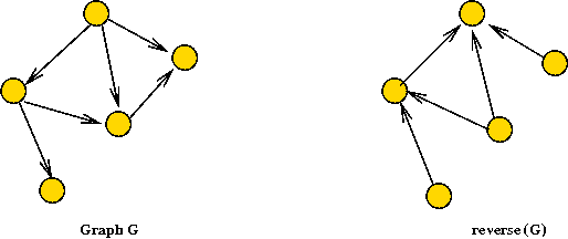
- First, we need to understand the reverse of a directed graph.
- Suppose G = (V,E) is a graph.
- G' = (V,E') is the reverse of G if
E'=E with the direction of edges reversed.
- Next, recall completion-order
lower completion order => closer to root
- The algorithm has two phases:
- First phase: find completion order on reverse graph using
standard DFS.
- Second phase: use a modified DFS on original graph in which
completion order is used as a priority.
- Let's describe the pseudocode first:
Algorithm: stronglyConnectedComponents (adjMatrix, n)
Input: A graph's adjacency matrix, number of vertices n.

1.    G' = reverse (G)
2.    completionOrder = depthFirstSearch (G')
3.    sortOrder = sort vertices in reverse order of completion           // Last to first.
4.    componentLabels = modifiedDepthFirstSearch (G, sortOrder)
5.    return componentLabels


Algorithm: modifiedDepthFirstSearch (adjMatrix, sortOrder)
Input: A graph's adjacency matrix, a sort (priority) order of vertices

1.   for i=0 to n-1
2.       visitOrder[i] = -1
3.   endfor
4.   visitCount = -1
5.   currentComponentLabel = -1

     // Look for an unvisited vertex and explore its tree.
6.   for i=0 to n-1
7.       v = sortOrder[i]                   // In order of completion of reverse search.
8.       if visitOrder[v] < 0
9.           currentComponentLabel = currentComponentLabel + 1
10.          modifiedDepthFirstMatrixRecursive (v)
11.      endif
12.  endfor
13.  return  componentLabels

Algorithm: modifiedDepthFirstMatrixRecursive (v)

     // Mark vertex v as visited and record component label.
1.   visitCount = visitCount + 1
2.   visitOrder[v] = visitCount
3.   componentLabel[v] = currentComponentLabel

     // Look for first unvisited neighbor.
4.   for i=0 to n-1
         u = sortOrder[i]                   // In order of completion of reverse search.
5.       if adjMatrix[v][u] > 0 and u != v
6.           if visitOrder[u] < 0
7.               depthFirstMatrixRecursive (u)
8.           endif
9.       endif
10.  endfor
Why does this work? The proof is in two parts.
Consider two vertices u and v.
Part (1): Suppose u and v are mutually
reachable:
- Suppose u is visited before v in the second-phase.
- Then, DFS will certainly visit v.
=> The algorithm reports both in the same component.
- The same holds if v is visited before u.
Part (2): Suppose u and v are reported in the
same component by the algorithm:
- Because u and v are in the same reported component,
they are part of a single tree
=> Let w be the root of this tree.
- Then w was visited before u and v.
=> w has a lower completion order than u and v.
(Store this fact for now).
- Next, observe that we reached u from w in
the second phase
=> there's a directed path from w to u in G.
=> there's a directed path from u to w in G'.
- Suppose there is no path from w to u in G'
(the reverse).
=> Then, the path from u to w in G' would
result in u having a higher completion order.
=> Contradiction.
- Thus, there is a path from w to u in G'.
=> There are paths in G from w to u and back.
The same argument shows that there is path from
w to v and back.
=> u and v are mutually reachable in G.
Tarjan's Algorithm:
- Some intuition:
- Consider what happens when we complete processing "3" in
- How can we identify the strong component "3, 4, 6"?
- First, there is no back edge that goes from "4, 6" to any node
"above" 3.
- Second, both "4" and "6" were visited in the descent from "3".
- But nodes "above" 3 will have a lower visitOrder.
=> keep track of lowest visitOrder reachable by a back edge
from a "potential component".
- How to mark vertices in a "component"?
- Build a stack.
- Place vertices on the stack as you recurse down.
- When coming back up the recursion, if you've identified
a component, all vertices in the component are going to be at
the top of the stack.
- Example above: "3, 4, 6" will be on the stack when returning
to "3".
- Another example: "0, 1, 2" will be at the top when returning
to "0".
(It won't be removed along the way back from "3" to "0").
- Pseudocode:
Algorithm: depthFirstMatrixRecursive (u, v)
Input: the vertex u from which this is being called, vertex v
       to be explored, adjMatrix is assumed to be global.

     // Mark vertex v as visited.
1.   visitCount = visitCount + 1
2.   visitOrder[v] = visitCount

     // Current lowest reachable:
3.   lowestReachable[v] = visitOrder[v];

     // Important: minLowestReachable is a local variable so that a
     // fresh version is used in each recursive call.
4.   minLowestReachable = lowestReachable[v];

     // Initialize stackTop to 0 outside. stackTop points to next available.
5.   stack[stackTop] = v;
6.   stackTop ++;

     // Look for first unvisited neighbor.
7.   for i=0 to n-1
8.       if adjMatrix[v][i] > 0 and i != v  // Check self-loop.

9.           if visitOrder[i] < 0
                 // If unvisited visit recursively.
10.              depthFirstMatrixRecursive (i)
11.          else if (i != u)  // Avoid trivial case.
                 // Identify back, down and cross edges ... (not shown)
12.          endif  // visitOrder < 0

13.          if lowestReachable[i] < minLowestReachable
14.              minLowestReachable = lowestReachable[i]
15.          endif

16.      endif  // adjMatrix[v][i] > 0
17.   endfor

     // We reach here after all neighbors have been explored.
     // Check whether a strong component has been found.
18.  if minLowestReachable < lowestReachable[v]
         // This is not a component, but we need to update the
         // lowestReachable for this vertex since its ancestors will
         // use this value upon returning.
19.      lowestReachable[v] = minLowestReachable
20.      return
21.  endif

     // We've found a component.
22.  do
         // Get the stack top.
23.      stackTop = stackTop - 1
24.      u = stack[stackTop];
         // We start currentStrongComponentLabel from "0".
25.      strongComponentLabels[u] = currentStrongComponentLabel;
         // Set this to a high value so that it does not affect
         // further comparisons up the DFS tree.
26.      lowestReachable[u] = numVertices;
27.  while stack[stackTop] != v

28.  currentStrongComponentLabel = currentStrongComponentLabel + 1
     // After returning from recursion, set completion order... (not shown)
Directed Acyclic Graphs (DAG's)
What are they?
- A DAG is a directed graph without a cycle
=> no path can cause you to revisit a vertex.
- Example:
- Example application: task scheduling
- A large activity consists of many related tasks.
- Some tasks need to occur before others.
=> typically a precedence relation among tasks.
- Represent task precedence using a DAG.
Sequential scheduling:
- Suppose the tasks represent programs that must be executed on a
sequential processor.
- Goal: find an execution sequence that does not violate
precedence constraints.
- Example: 3 0 1 2 5 4 6 7
- Note: 4 0 1 2 5 3 6 7 violates precedence requirements.
Topological sort:
- A topological sort of a DAG is a sequence of vertices
that:
- does not violate precedence;
- contains all the vertices.
- A simple (the "classic") algorithm:
- Find a vertex that has no predecessors (zero in-degree)
(there must be one, or it's not a DAG).
- Add this to the sequence.
- Remove it from the graph.
- In removing, adjust the in-degree of every neighbor of the
removed vertex.
- Repeat.
In-Class Exercise 7.11:
Apply the classic algorithm to the above example.
Using depth-first search:
- Key observation: the vertex whose completion occurs
first in depth-first search can be placed last in the sequence.
- Why? It has no successors (descendants in the DFS tree).
- Steps:
- Examine completionOrder in depth-first search.
- Place first vertex to complete at end of sequence.
- Remove it from the graph.
- Place next vertex to complete in next-to-last in sequence.
- ... and so on ...
- Note: after DFS "completes" a vertex, the vertex is never
seen again
=> no need to remove it from graph!
- Example:
Pseudocode:
- We only need to record topological sort order every time a
completion occurs.
- Partial pseudocode:
Algorithm: depthFirstMatrixRecursive (u, v)
Input: the vertex u from which this is being called, vertex v
       to be explored, adjMatrix is assumed to be global.

     // Mark vertex v as visited.
1.   visitCount = visitCount + 1
2.   visitOrder[v] = visitCount

     // Look for first unvisited neighbor and recurse
3.   for i=0 to n-1
          // ... (same as before, not shown) ...
4.   endfor

     // After returning from recursion, set completion order:
5 .  completionCount = completionCount + 1
6.   completionOrder[v] = completionCount

     // Set topological sort order.
     // Initialize topSortCount to -1 outside this method
7.   topSortCount = topSortCount + 1
8.   topSortOrder[topSortCount] = v