Module 10: Combinatorial Optimization Problems,
State Spaces and Local Search
Optimization Problems
What are they?
- An optimization problem has "input" and a "measure"
=> different solutions possible, each of different value
=> Goal: find the "best" solution.
- The "measure" is sometimes called an objective function.
- Some problems have constraints: not all potential solutions
are "acceptable".
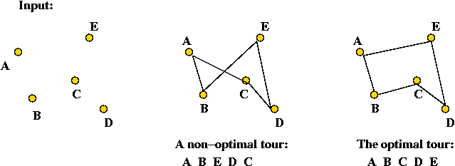
Example: the Travelling Salesman Problem (TSP)
- Input: a collection of points (representing cities).
- Goal: find a tour of minimal length.
Length of tour = sum of inter-point distances along tour

- Details:
- Input will be a list of n points, e.g., (x0, y0),
(x1, y1), ..., (xn-1, yn-1).
- Solution space: all possible tours.
- "Cost" of a tour: total length of tour.
=> sum of distances between points along tour
- Goal: find the tour with minimal cost (length).
- Note: strictly speaking, we have defined the Euclidean TSP.
=> There is also a graph version that we will not consider

- Applications:
- Logistics: trucking and delivery problems.
- Machine operation (e.g., drilling a collection of holes)
In-Class Exercise 10.1:
For an n-point problem, what is the size of the solution space
(i.e., how many possible tours are there)?
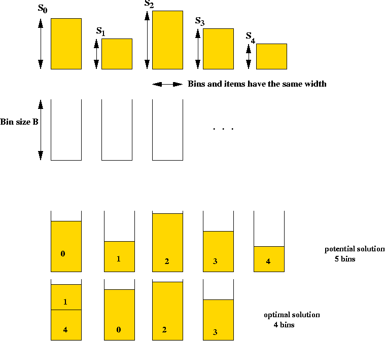
Example: the Bin Packing Problem (BPP)
- Input: a collection of items and unlimited bins.
- Goal: pack the items into as few bins as possible.

- Details:
- Input is a list of n integer bin sizes s0,
s1, ..., sn-1 and an integer bin size B.
- Solution space: all feasible packings
=> all assignments of items to bins such that no bin
overflows. (A constraint).
=> sum of sizes of items assigned to each bin is at most B.
- Goal: find the assignment that uses the fewest bins.
- Note: assume si < B.
- Alternate description:
- Item sizes: s0, s1, ...,
sn-1
where si < B.
- Define the assignment function:
| dij |
= |
1,
0, |
if item i is placed in bin j
otherwise |
- B = bin size.
- Goal: minimize k, the number of bins
such that:
- For each j,
s0dij + ... + sn-1dij < B
(all items assigned to bin j fit into the bin)
- For each i, dij + ... +
dij = 1
(each item is assigned to a bin)
In-Class Exercise 10.2:
Consider the following Bin Packing problem: there are three items with sizes
1, 2 and 3 respectively, and a bin size of 6.
Enumerate all possible assignments.
Example: Quadratic Programming Problem
- Input: n coefficients a0, a1,
..., an-1.
- Goal: minimize a0x02 +
a1x12 + ...
+ an-1xn-12.
- Constraint: x0 + ... + xn-1 = K
- Here, each xi is real-valued.
- Example:
Minimize 3 x02 + 4 x12
Such that x0 + x1 = 10
Types of optimization problems:
- The Quadratic Programming problem is very different
from both TSP and BPP.
- TSP and BPP are similar is some structural respects.
- Two fundamental types of problems:
- Discrete optimization problems: finite or countable solution space.
=> usually finite number of potential solutions.
- Continuous optimization problems: uncountable solution space
=> variables are real-valued.
- Examples:
- Discrete: TSP, BPP
- Continuous: Quadratic Programming problem.
- We will focus on discrete optimization problems.
Problem Size and Execution Time
Problem size:
- Typically, the "size" of a problem is the space required to
specify the input:
- Example: TSP
=> For an n-point problem, space required is: O(n).
- Example: BPP
=> For an n-item BPP, O(n) space is required.
- Non-Euclidean TSP
- Recall: a graph is given
=> required to use only edges in the graph.
- A graph with n vertices can have
O(n2) edges
=> O(n2) space required for input.
- Consider this TSP example:
- Input: "The points are n equally spaced points on the
circumference of the unit circle".
- How much space is required for an input of 10-points? For 1000-points?
=> O(1) !
- The above example is not general
=> we need O(n) space (worst-case) to describe
any TSP problem.
- Terminology: instance
- A problem instance is a particular problem (with the
data particular to that problem).
- Example: TSP on the 4 points (0, 1), (0.5, 0.6),
(2.5, 3.7) and (1, 4).
=> an instance of size 4.
- Another instance: TSP on the 5 points (0, 1), (0.5, 0.6),
(2.5, 3.7), (1, 4) and (6.8, 9.1).
=> an instance of size 5.
Execution time of an algorithm:
- What we expect of an algorithm:
- An algorithm is given its input and then executed.
- The algorithm should produce a candidate solution or report
that no solutions are possible.
- Example: TSP
- An algorithm is given the set of input points.
- The algorithm should output a tour after execution.
- Example: BPP
- An algorithm is given the item sizes and bin size as input.
- The algorithm should output an assignment
(Or report that some items are too large to fit into a bin).
- Output size:
- Example: TSP
- Output is a tour
=> O(n) output for n points.
- Example: BPP
- Output is an assignment.
- If assignment is specified as the function
| dij |
= |
1,
0, |
if item i is placed in bin j
otherwise |
then output could be as large as O(n2).
- Execution time:
=> Total execution time includes processing input and writing output.
Consider these two algorithms for TSP:
- Algorithm 1:
- Initially the set P = {0, ..., n-1 } and the set
Q is empty.
- Move 0 from P to Q.
- Repeat the following until P is empty:
- Suppose k was the point most recently added to
Q.
- Find the point in P closest to k and move
that to Q.
- Output points in the order in which they were added to Q.
- Algorithm 2:
- Generate a list of all possible tours and place in an array
(of tours).
- Scan array and evaluate the length of each tour.
- Output the minimum-length tour.
In-Class Exercise 10.3:
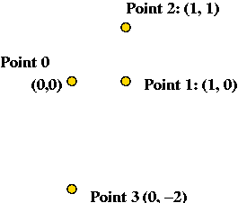
Consider the following 4 input points: (0,0), (1,0), (1,1) and
(0,-2).

- Show the steps in executing each algorithm on this input.
- What is the complexity (execution time) of Algorithm 1 on an
input of size n?
- What is the complexity of Algorithm 2 on an
input of size n?
Polynomial vs. exponential complexity:
- An algorithm has polynomial complexity or runs in
polynomial time if its execution time can be bounded by a polynomial function
of its input size.
- Example: An algorithm takes O(n3) (worst-case) on input of size
n
=> algorithm is a polynomial-time algorithm.
- Requirements for the polynomial:
- Highest power in the polynomial should be a constant (i.e.,
not dependent on n.
- Polynomial should be finite (not an infinite sum of terms).
- Algorithms that run slower-than-polynomial are said to have
exponential complexity:
- Typically, the (worst-case) running time is something like
O(an).
- Note: factorials have (like O(n!)) have exponential
complexity
=> From Stirling's formula: n! = O(sqrt(n) * (cn)n).
In-Class Exercise 10.4:
Which of these are polynomial-time algorithms?
- Algorithm 0 runs in time O( (n2 + 3)4 ).
- Algorithm 1 runs in time O(n log(n)).
- Algorithm 2 runs in time O(nn).
- Algorithm 3 runs in time O(nlog(n)).
- Algorithm 4 runs in time O( (log n)3 ).
Preview of things to come:
- Many important optimization problems are
discrete optimization problems.
- For these problems:
- It's easy to find simple algorithms of polynomial complexity
=> but that are not guaranteed to find optimal solutions.
- The only algorithms that guarantee optimality take
exponential time.
Combinatorial Optimization Problems
A combinatorial optimization problem is:
- A set of states or candidate solutions S = {
s0, s1, ..., sm} .
- A cost function C defined on the states
=> C(s) = cost of state s.
- Goal: find the state with the least cost.
Example: TSP
- Each instance of TSP is a combinatorial optimization problem.
- Example: the 4-point TSP problem with points (0,1), (1,0),
(2,3) and (3,5)
- Does this have a set of "states" or "candidate solutions"?
=> Yes: S = { all possible tours }
= { [0 1 2 3], [0 1 3 2], [0 2 1 3] }
- Is there a well-defined cost function on the states?
=> Yes: C(s) = length of tour s
e.g., C([0 1 2 3]) = dist(0,1) + dist(1,2) + dist(2,3) + dist(3,0).
- Is the goal to find the least-cost state?
=> Yes: find the tour with minimal length.
Example: BPP
- States: all possible assignments of items to bins.
- Cost function: C(s) = number of bins used in state s.
- Goal: find the state that uses the least bins (minimal-cost state).
In-Class Exercise 10.5:
Which of these, if any, are combinatorial optimization problems?
Identify the state space for each.
- Given a connected, weighted graph, find the minimum-spanning tree.
- Given a connected graph, discover whether it has a Hamiltonion tour.
(Recall: a Hamiltonian tour is a tour that passes through
each vertex exactly once.)
- Find the values of x1 and x2
that minimizes the function
f(x1, x2)
= x12 + x22
such that 3x1+2x2=100
Size of a combinatorial optimization problem:
- The input is usually of size O(n) or O(n2).
- TSP: list of n points.
- BPP: n item sizes and one bin size.
- Graph-based TSP: n vertices and up to
O(n2) edges.
- MST: n vertices and up to
O(n2) edges.
- The state-space is usually exponential in size:
- TSP: all possible tours.
- BPP: all possible assignments of items to bins.
- MST: all possible spanning trees.
- The output is usually of size O(n) or
O(n2)
- TSP: a tour of size O(n)
- BPP: an assignment (matrix) of size O(n2).
- MST: an adjacency matrix of size O(n2).
Greedy Algorithms
Key ideas:
- For many combinatorial optimization problems (but not all!), it
is easy to build a candidate solution quickly.
- Use problem structure to put together a candidate solution step-by-step.
- At each step: "do the best you can with immediate information"
- Greedy algorithms are usually O(n) or O(n2).
Example: TSP
- Greedy Algorithm:
- Initially the set P = {0, ..., n-1 } and the set
Q is empty.
- Move 0 from P to Q.
- Repeat the following until P is empty:
- Suppose k was the point most recently added to
Q.
- Find the point in P closest to k and move
that to Q.
- Output points in the order in which they were added to Q.
- What is "greedy" about this?
- At each step, we add a new point to the existing tour.
- The new point is selected based on how close it is to
previous point.
Greedy => no backtracking.
- Execution time: O(n2) (each step requires
an O(n) selection).
- Solution quality: not guaranteed to find optimal solution.
Example: BPP
- Greedy Algorithm:
- Let A = { all items }
- Sort A in decreasing order.
- At each step until A is empty:
- Remove next item in sort-order from A.
- Find first-available existing bin to fit item.
- If no existing bin can fit the item, create a new bin and
place item in new bin.
- Running time: O(n log(n)) for sort and
O(n2) for scanning bins at each step (worst-case).
=> O(n2)
- Solution quality: not guaranteed to find optimal solution.
Example: MST (Minimum Spanning Tree)
- Greedy Algorithm: (Kruskal)
- Sort edges in graph in increasing order of weight.
- Process edges in sort-order:
- If adding the edge causes a cycle, discard it.
- Otherwise, add the edge to the current tree.
- Complexity: O(E log(E)) for sorting, and O(E
log(V)) for processing the edges with union-find.
=> O(E log(E)) overall.
- Solution quality: finds optimal solution.
About greedy algorithms:
- For many problems, it's relatively easy to pose a greedy algorithm.
- For a few problems (e.g., MST), the greedy algorithm produces the
optimal solution.
- For some problems (e.g. BPP), greedy algorithms produce "reasonably
good" solutions (worst-case).
- For some problems (e.g. BPP), greedy algorithms produce "excellent"
solutions (in practice).
- For some problems (e.g., Hamiltonian tour), greedy
algorithms are of no help at all.
Walking around the State Space
Consider the following two algorithms for TSP:
- Algorithm 1:
     // Start with input-order tour:
1.   s = initial tour 0,1,...,n-1

     // Record current best tour.
2.   min = cost(s)
3.   minTour = s

     // Repeat a large number of times:
4.   for i=1 to very-large-number
         // Create a random tour from scratch.
5.       s = generate random tour
         // See if it's better than our current best.
6.       if cost(s) < min
7.           min = cost(s)
8.           minTour = s
9.       endif
10.  endfor

     // Return best tour found.
11.  return minTour
- Algorithm 2:
     // Start with input-order tour:
1.   s = initial tour 0,1,...,n-1

     // Record current best tour.
2.   min = cost(s)
3.   minTour = s

     // Repeat a large number of times:
4.   for i=1 to very-large-number
         // Use current tour s to create next tour
5.       Pick two random points in s;
6.       s = tour you get by swapping the two selected points in s
         // See if it's better than our current best.
7.       if cost(s) < min
8.           min = cost(s)
9.           minTour = s
10.      endif
11.  endfor

     // Return best tour found.
12.  return minTour
In-Class Exercise 10.6:
Start with a 5-point TSP problem. Use some physical solution
to creating randomness (e.g, flip coins) and emulate the above two
algorithms for a few steps.
- Observe:
Each algorithm "walks around" the state space in some random fashion.
- Neighborhood:
- Define N(s) = Neighborhood(s) = { all states you can get to from
s} in any particular iteration using one of the above algorithms.
- Example: 4-point problem
- N (0123) = { all possible tours } in Algorithm 1.
- N (0123) = { 0213, 0321, 0132 } in Algorithm 2.
- A neighborhood is polynomial if the size of each
neighborhood can be bounded by a polynomial of the input size.
In-Class Exercise 10.7:
For an n-point TSP instance, what is the size of a
neighborhood in each of the above algorithms?
A different way of writing the code:
- Consider this generic "walk" in state-space:
Algorithm: stateSpaceWalk (points)
Input: n points in TSP problem
1.   s = initial tour 0,1,...,n-1
2.   min = cost(s)
3.   minTour = s
4.   for i=1 to very-large-number
         // Let method "nextState" produce the next state
5.       s = nextState(s)
6.       if cost(s) < min
7.           min = cost(s)
8.           minTour = s
9.       endif
10.  endfor
11.  return minTour
- We have seen two different nextState function's:
- Algorithm 1 above:
Algorithm: nextState (s)
Input: current state s
    // Ignore s and generate an arbitrary tour
1.  t = Generate a random tour
2.  return t
- Algorithm 2 above:
Algorithm: nextState (s)
Input: current state s
1.  t = s
2.  Pick any two random points in t
3.  Swap them.
4.  return t
Reachability:
- A "nextState" function is reachable if, from the start state,
you can eventually reach every other state by walking around long enough.
- Both "nextState" functions above are reachable.
In-Class Exercise 10.8:
Can you think of a nextState function that is not "reachable"?
Greedy Local Search
Key ideas:
- A local search algorithm:
- An algorithm for a combinatorial optimization problem.
- Uses a "nextState" function to roam around the state space.
- Records the "best-solution-seen-so-far" while roaming.
- A greedy local search algorithm:
- Has little to do with "greedy algorithms" described earlier.
- Uses a more intelligent "nextState" function
=> it examines the neighborhood, and selects the best state in
the neighborhood.
Example: greedy local search for TSP
- Idea:
- Generate a neighborhood N(s) for the current state s
- Pick the "best" (lowest-cost) state in N(s) as the
next-state.
- Repeatedly pick "best" neighbors until no neighbor is better.
- Pseudocode:
Algorithm: TSPGreedyLocalSearch (points)
Input: array of points

     // Start with any tour, e.g., in input order
1.   s = initial tour 0,1,...,n-1

     // Repeatedly find a "neighboring" tour, as long as the neighbor is better.
2.   repeat
3.       min = cost(s)
4.       minTour = s
         // Use "greedy" approach in finding a new state to walk to.
5.       s = greedyNextState(s)
6.   until cost(s) > min

     // Output best tour seen.
7.   return minTour

Output: best tour found by algorithm
Algorithm: greedyNextState (s)
Input: a tour s, an array of integers

     // Start with current tour.
1.   min = cost (s)
2.   bestNeighbor = s

     // Generate all possible neighbors by swapping two elements in s.
     // Note: go through all possible i and j systematically - O(n2) combinations
3.   for each i and j
4.       s' = swap i-th and j-th points in s
5.       if cost (s') < min
6.           min = cost (s')
7.           bestNeighbor = s'
8.       endif
9.   endfor

     // Return best one found.
10.  return bestNeighbor

Output: a tour (the best neighboring tour, using only swaps)
Greedy local search for BPP:
- Start with any assignment of items to bins.
- At each step, find the least-cost "neighboring assignment"
and make that the next assignment.
- Repeat this process until no neighbor is better.
- Computing a "neighbor":
- The current state is an assignment of items to bins.
- Try swaps between all possible pairs of bins, i and j.
- For a particular pair of bins i and j, pick an item in each
randomly and swap them.
Non-uniqueness of greedy-local-search:
- There is no "best way" to define greedy local search for a problem.
- It is possible to devise many different heuristics for
greedy local search.
- Example: alternative greedy heuristic for TSP
- Given the current tour s, consider all possible next
tours you can get by a 3-way swap.
- Example: alternative greedy heuristic for BPP
- Given current assignment, lay out items in order of
bins. Then, swap items and return to bins in first-fit order.
In-Class Exercise 10.9:
Download this
template
and implement the following variation of greedy-local-search:
- Instead of trying all possible pairs (which takes
O(n2) time, we will use an O(n)-neighborhood.
-
Given the current tour, pick a random point i in the current tour.
-
Then, try all possible other points j ( j != i) to get
n-1 pairs (i,j).
- Try a swap of i and j for each of these pairs, and pick the best one.
- Return the tour resulting from the best such swap as the nextState.
Local Optima and Problem Landscape
Local optima:
- Recall: greedy-local-search generates one state (tour) after
another until no better neighbor can be found
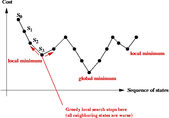
=> does this mean the last one is optimal?
- Observe the trajectory of states:

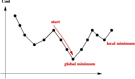
- There is no guarantee that a greedy local search can find the
(global) minimum.
- The last state found by greedy-local-search is a local minimum.
=> it is the "best" in its neighborhood.
- The global minimum is what we seek: the least-cost
solution overall.
- The particular local minimum found by greedy-local-search
depends on the start state:

Problem landscape:
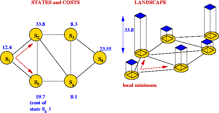
- Consider TSP using a particular local-search algorithm:
- Suppose we use a graph where the vertices represent states.
- An edge is placed between two "neighbors"
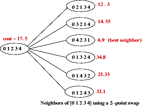
e.g., for a 5-point TSP the neighbors of [0 1 2 3 4] are:

- The cost of each tour is represented as the "weight" of each vertex.
- Thus, a local-search algorithm "wanders" around this graph.
- Picture a 3D surface representing the cost above
the graph.
=> this is the problem landscape for a particular problem and
local-search algorithm.

- A large part of the difficulty in solving combinatorial
optimization problems is the "weirdness" in landscapes
=> landscapes often have very little structure to exploit.
- Unlike continuous optimization problems, local shape in the
landscape does NOT help point towards the global minimum.
Climbing out of local minima:
- A local-search algorithm gets "stuck" in a local minimum.
- One approach: re-run local-search many times with different
starting points.
- Another approach (next): help a local-search algorithm
"climb" out of local minima.
Simulated Annealing
Background:
- What is annealing?
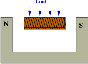
- Annealing is a metallurgic process for improving the
strength of metals.
- Key idea: cool metal slowly during the forging process.
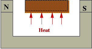
- Example: making bar magnets:
- Wrong way to make a magnet:
- Heat metal bar to high temperature in magnetic field.

- Cool rapidly (quench):

- Right way: cool slowly (anneal)
- Why slow-cooling works:
- At high heat, magnetic dipoles are agitated and move around:

- The magnetic field tries to force alignment:

- If cooled rapidly, alignments tend to be less than optimal
(local alignments):

- With slow-cooling, alignments are closer to optimal (global alignment):

- Summary: slow-cooling helps because it gives molecules more time
to "settle" into a globally optimal configuration.
- Relation between "energy" and "optimality"
- The more aligned, the lower the system "energy".
- If the dipoles are not aligned, some dipoles' fields will conflict
with others.
- If we (loosely) associate this "wasted" conflicting-fields
with energy
=> better alignment is equivalent to lower energy.
- Global minimum = lowest-energy state.
- The Boltzmann Distribution:
- Consider a gas-molecule system (chamber with gas molecules):

- The state of the system is the particular snapshot (positions
of molecules) at any time.
- There are high-energy states:

and low-energy states:

- Suppose the states s1, s2, ...
have energies E(s1), E(s2), ...
- A particular energy value E occurs with probability
P[E] = Z e-E/kT
where Z and k are constants.
- Low-energy states are more probable at low temperatures:
- Consider states s1 and s2
with energies E(s2) > E(s1)
- The ratio of probabilities for these two states is:
r = P[E(s1)] / P[E(s2)]
= e[E(s2) - E(s1)] / kT
= exp ([E(s2) - E(s1)] / kT)
In-Class Exercise 10.10:
Consider the ratio of probabilities above:
- Question: what happens to r as T increases to infinity?
- Question: what happens to r as T decreases to zero?
What are the implications?
Key ideas in simulated annealing:
- Simulated annealing = a modified local-search.
- Use it to solve a combinatorial optimization problem.
- Associate "energy" with "cost".
=> Goal: find lowest-energy state.
- Recall problem with local-search: gets stuck at local minimum.
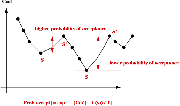
- Simulated annealing will allow jumps to higher-cost states.
- If randomly-selected neighbor has lower-cost, jump to it (like
local-search does).
- If randomly-selected neighbor is of higher-cost
=> flip a coin to decide whether to jump to higher-cost state
- Suppose current state is s with cost C(s).
- Suppose randomly-selected neighbor is s' with cost C(s') > C(s).
- Then, jump to it with probability
e-[C(s') - C(s)] / kT
- Decrease coin-flip probability as time goes on:
=> by decreasing temperature T.
- Probability of jumping to higher-cost state depends on cost-difference:

Implementation:
- Pseudocode: (for TSP)
Algorithm: TSPSimulatedAnnealing (points)
Input: array of points

     // Start with any tour, e.g., in input order
1.   s = initial tour 0,1,...,n-1

     // Record initial tour as best so far.
2.   min = cost (s)
3.   minTour = s

     // Pick an initial temperature to allow "mobility"
4.   T = selectInitialTemperature()

     // Iterate "long enough"
5.   for i=1 to large-enough-number
           // Get potential next state using greedy-local-search.
6.         s' = randomNextState (s)
           // If it's better, then jump to it.
7.         if cost(s') < cost(s)
8.             s = s'
               // Record best so far:
9.             if cost(s') < min
10.                min = cost(s')
11.                minTour = s'
12.            endif
13.        else if expCoinFlip (s, s')
               // Jump to s' even if it's worse.
14.            s = s'
15.        endif       // Else stay in current state.
           // Decrease temperature.
16.        T = newTemperature (T)
17.  endfor

18.  return minTour

Output: best tour found by algorithm
Algorithm: randomNextState (s)
Input: a tour s, an array of integers

    // ... Swap a random pair of points ...

Output: a tour
Algorithm: expCoinFlip (s, s')
Input: two states s and s'

1.   p = exp ( -(cost(s') - cost(s)) / T)
2.   u = uniformRandom (0, 1)
3.   if u < p
4.       return true
5.   else
6.       return false

Output: true (if coinFlip resulted in heads) or false
- Implementation for other problems, e.g., BPP
- The only thing that needs to change: define a
nextState method for each new problem.
- Also, some experimentation will be need for the temperature schedule.
Temperature issues:
- Initial temperature:
- Need to pick an initial temperature that will accept large
cost increases (initially).
- One way:
- Guess what the large cost increase might be.
- Pick initial T to make the probability 0.95 (close
to 1).
- Decreasing the temperature:
- We need a temperature schedule.
- Several standard approaches:
- Multiplicative decrease:
Use T = a * T, where a is a constant like 0.99.
=> Tn = an.
- Additive decrease:
Use T = T - a, where a is a constant like 0.0001.
- Inverse-log decrease:
Use T = a / log(n).
- In practice: need to experiment with different temperature
schedules for a particular problem.
Analysis:
- How long do we run simulated annealing?
- Typically, if the temperature is becomes very, very small
there's no point in further execution
=> because probability of escaping a local minimum is miniscule.
- Unlike previous algorithms, there is no fixed running time.
- What can we say theoretically?
- If the inverse-log schedule is used
=> Can prove "probabilistic convergence to global minimum"
=> Loosely, as the number of iterations increase, the
probability of finding the global minimum tends to 1.
In practice:
- Advantages of simulated annealing:
- Simple to implement.
- Does not need much insight into problem structure.
- Can produce reasonable solutions.
- If greedy does well, so will annealing.
- Disadvantages:
- Poor temperature schedule can prevent sufficient exploration
of state space.
- Can require some experimentation before getting it to work well.
- Precautions:
- Always re-run with several (wildly) different starting solutions.
- Always experiment with different temperature schedules.
- Always pick an initial temperature to ensure high probability
of accepting a high-cost jump.
- If possible, try different neighborhood functions.
- Warning:
- Just because it has an appealing origin, simulated annealing
is not guaranteed to work
=> when it works, it's because it explores more of the state
space than a greedy-local-search.
- Simply running greedy-local-search on multiple starting
points may be just as effective, and should be experimented with.
Variations:
- Use greedyNextState instead of the nextState function above.
- Advantage: guaranteed to find local minima.
- Disadvantage: may be difficult or impossible to climb out of
a particular local minimum:
- Suppose we are stuck at state s, a local minimum.
- We probabilistically jump to s', a higher-cost state.
- When in s', we will very likely jump back to
s (unless a better state lies on the "other side").
- Selecting a random next-state is more amenable to exploration.
=> but it may not find local minima easily.
- Hybrid nextState functions:
- Instead of considering the entire neighborhood of 2-swaps,
examine some fraction of the neighborhood.
- Switch between different neighborhood functions during iteration.
- Maintain "tabu" lists:
- To avoid jumping to states already seen before, maintain a
list of "already-visited" states and exclude these from each neighborhood.
In-Class Exercise 10.11:
Download this
template
and implement simulated annealing using the neighborhood function of
Exercise 10.9. The main-loop as well as the temperature schedule is
already in the template.
