Module 8: Science and Engineering Applications - Part I

Objectives

By the end of this module, for simple programs with real numbers, you will be able to:

Apply loops/variables to evaluating sequences and sums.
Demonstrate plotting of functions.
Demonstrate straight-line fit for some data.
Demostrate the use of finite difference approximation for derivatives.

Sequences, Series and Limits

One of the most important ideas in mathematics is the idea of a limit:

Let X₁, X₂, ..., X_n, ... be a sequence of real numbers.
A limit explores the idea of what the sequences tends towards.
Example: suppose X_n = 1/n.
=> Then, clearly X_n gets closer to 0 as n → ∞.
Note: there is no n for which X_n=0.
We say lim_n→∞ 1/n = 0.
In words: "The limit of 1/n as n goes to infinity is zero".

In-Class Exercise 1: Suppose a is some real number greater than 0. What is lim_n→∞ aⁿ? Is this true for, say, a = 1.00001?

However, the limit is less clear for this sequence: X_n = (1 + 1/n)ⁿ
Let's write a program to compute successive elements of this sequence:

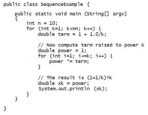
In-Class Exercise 2: Edit, compile and execute the program. Try larger values of n. What does the sequence appear to converge to?

Let's look at how a sequence can be used to estimate another famous constant: π

We'll use the so-called Gregory-Leibniz series:
π = 4 (1 - 1/3 + 1/5 - 1/7 + 1/9 + ....)
Let's do this in steps. First, suppose we had to compute
1 + 1/3 + 1/5 + 1/7 + 1/9 + ....

Some pseudocode:

        sum = 0
	for i=1 to k {
           sum = sum + 1/(2*i-1)
        }

Next, how do we alternate the sign? Here's one way:

        sum = 0
	sign = 1
	for i=1 to k {
           sum = sum + sign/(2*i-1)
	   sign = -sign;
        }

Now let's put this all into code to print out the first n terms:

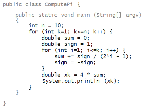
In-Class Exercise 3: Edit, compile and execute the program. Try larger values of n to see how quickly it converges to π. When k=4 in the outerloop, trace through the execution inside the outerloop.

Let's look at a third famous constant: Φ, the golden ratio.

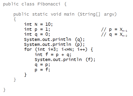
Recall the definition of the Fibonacci sequence: X_n = X_n-1 + X_n-2.
The starting values: X₀=0, X₁ = 1.
We wrote a program to print out successive Fibonacci numbers:
Consider the sequence Y_n = X_n / X_n-1.
That is, the ratio of successive Fibonacci terms.

In-Class Exercise 4: Modify the above program to compute this ratio. What does it appear to converge to? Can you derive this limit mathematically? [Hint: Use the definition X_n = X_n-1 + X_n-2. ]

Zeno's paradox:

Zeno was a Greek philosopher who is famous for creating several apparent paradoxes.
His most famous one: the hare and the tortoise
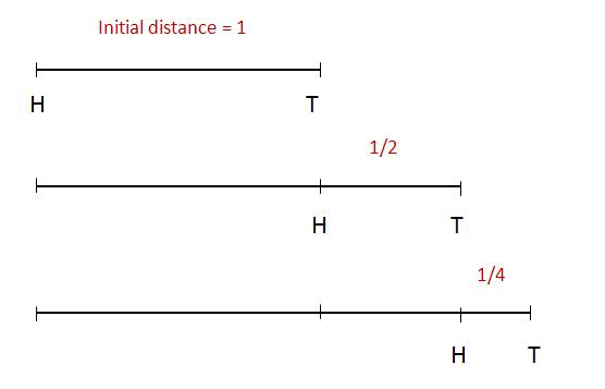
- Suppose a hare and tortoise are separated by 1 unit of distance.
- Suppose hare is twice as fast as tortoise.
In the time the hare covers 1 unit, the tortoise has moved foward 1/2 unit.
In the time taken to cover this 1/2 unit, the tortoise has moved forward 1/4 unit ... etc.
Zeno claimed that by the time the hare catches up, the tortoise will have traveled:
1/2 + 1/4 + 1/8 + ....
An infinite sum
Zeno's paradox: the hare will never catch up.
Let's resolve this by writing a program to compute
1/2 + 1/4 + 1/8 + ....
Such a sum is often called a series:
It can be written as a sequence. Define
X_n = 1/2 + 1/4 + 1/8 + .... + 1/2ⁿ
Then, we are interested in
lim_n→∞ X_n

Let's write a program to compute this for any n:

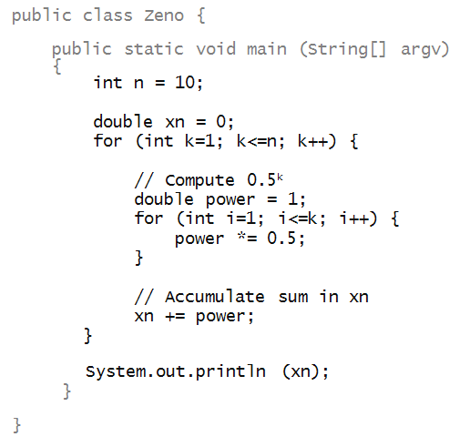
Note: in the program above, xn is a variable name.
=> We could just as easily have called it anything else.

In-Class Exercise 5: What does the series appear to converge to? Can you derive this limit mathematically?

In-Class Exercise 6: Suppose X_n = 1 + 1/2 + 1/3 + 1/4 + .... + 1/n. Write a program to compute this sum for different values of n What can you say about its limit?

Functions

Let's now work with functions. To start with, let's plot the function f(x) = x³/100 in the range x ε [0,10].

In-Class Exercise 7: Download DrawTool.java and FunctionExample.java. Then, compile and execute FunctionExample.java. Edit the file FunctionExample.java to increase to 100 the number of points at which the function is computed - this should produce a smoother curve.

Next, let's work with some real data

Consider the following data:

x	*f(x)*
8.33	1666.67
22.22	3666.67
23.61	4833.33
30.55	5000
36.81	5166.67
47.22	8000
69.44	11333.33
105.56	19666.67

Let's write code to display this data:

public class FunctionData {

    public static void main (String[] argv)
    {
	DrawTool.display ();
	DrawTool.setXYRange (0, 110, 0, 20000);

	double x = 8.33; 
	double f = 1666.67;
	DrawTool.drawPoint (x,f);

	x = 22.2;  f = 3666.67;
	DrawTool.drawPoint (x,f);

	x = 23.61;  f = 4833.33;
	DrawTool.drawPoint (x,f);

	x = 30.55;  f = 5000;
	DrawTool.drawPoint (x,f);

	x = 36.81;  f = 5166.67;
	DrawTool.drawPoint (x,f);

	x = 47.22;  f = 8000;
	DrawTool.drawPoint (x,f);

	x = 69.44;  f = 11333.33;
	DrawTool.drawPoint (x,f);

	x = 105.56;  f = 19666.67;
	DrawTool.drawPoint (x,f);
    }

}

Notice that we had to adjust the default x and y range.

In-Class Exercise 8: Edit, compile and execute FunctionData.java. Then, try to estimate the slope of a line that would approximately "fit" the points. Use the DrawTool.drawLine method to draw a line with your estimated slope. For example, if your estimated slope is m, you would add this to your program:

    DrawTool (0,0, 110, m*110);

Fitting a line to data:

Suppose the given data is slightly "noisy"
=> There are measurement errors.
We want to find the best line that fits the data.
For the above example, let's assume the line is: y = mx + c.
For the above data, let's assume c=0.
Suppose we guessed m=150. Then, why would this better than, say, m=140?

In-Class Exercise 9: How does one evaluate how best a given line fits some points?

For a given x, the data value is f(x).
The predicted value, on the other hand, is: mx.
We could say that the error for a given x is: f(x)-mx.

In-Class Exercise 10: With m=140, compute the error for some of the x values. The preferred way of computing the error is to use the square (f(x) - mx)². Why is this?

Now, let's write code to compute the total error, given a slope m.

	    sum = 0;
	    x = 8.33; f = 1666.67;
	    double error = (m*x-f) * (m*x-f);
	    sum += error;

	    x = 22.2;  f = 3666.67;
	    error = (m*x-f) * (m*x-f);
	    sum += error;

	    x = 23.61;  f = 4833.33;
	    error = (m*x-f) * (m*x-f);
	    sum += error;

	    x = 30.55;  f = 5000;
	    error = (m*x-f) * (m*x-f);
	    sum += error;

	    x = 36.81;  f = 5166.67;
	    error = (m*x-f) * (m*x-f);
	    sum += error;

	    x = 47.22;  f = 8000;
	    error = (m*x-f) * (m*x-f);
	    sum += error;

	    x = 69.44;  f = 11333.33;
	    error = (m*x-f) * (m*x-f);
	    sum += error;

	    x = 105.56;  f = 19666.67;
	    error = (m*x-f) * (m*x-f);
	    sum += error;

	    System.out.println (sum);

In-Class Exercise 11: Use this to compute the total error when m=160.

What we'd like to do: use a loop to try different values of m

     for m=start to end {
        Use slope m
        Compute the error from the data using y=mx
        Print the error
     }

In-Class Exercise 12: Add a for-loop to print the total error for values of values of m in the range 160-190, in increments of 1. What is the slope that results in the least error? Plot a line along with the points using this slope.

In-Class Exercise 13: The data is from a world-changing paper published in 1929. Use a websearch to discover what the data is and why it changed the world.

Using animation for visualization

We will explore the use of visualization for problems in motion:

Consider an object (say, car) that's moving at velocity v meters/second.
Then, the distance traveled after t units of time is: d = vt meters.
Similarly, consider a ball that's dropped from a height of 100 meters.
The height after t seconds is: h = 100 - ½gt².
(Here, g = 9.8).

Let's visualize both using our drawing tool:

public class MotionExample {

    public static void main (String[] argv)
    {
	DrawTool.display ();
	DrawTool.setXYRange (0,100, 0,100);

	DrawTool.startAnimationMode ();
	double v = 10;
	for (double t=0; t<=10; t+=0.1) {
	    double d = v*t;
	    double h = 100 - 0.5*9.8*t*t;
	    DrawTool.writeTopValue (t);
	    DrawTool.setPointColor ("blue");
	    DrawTool.drawPoint (d, 0);
	    DrawTool.setPointColor ("red");
	    DrawTool.drawPoint (70, h);
	    DrawTool.animationPause (100);
	}
	DrawTool.endAnimationMode ();
    }

}

In-Class Exercise 14: Edit, compile and execute the above program. Make sure DrawTool.java is in the same directory. Guess at the velocity v needed to create a collision between the two objects. At what time would this occur?

Estimating derivatives

What is a derivative?

Consider a function f(x).
Let Δ represent a number, typically a small number relative to x.
Now define, for any x the quantity
(f(x+Δ) - f(x)) / Δ
Note: for any fixed Δ, the above quantity depends on x
=> It's a function of x.
We can call it g(x):
g(x) = (f(x+Δ) - f(x)) / Δ
Consider our earlier example: f(x) = x³/100.

Here's a small program to compute g(x):

public class Derivative {

    public static void main (String[] argv)
    {
	double x = 1;
	double f = x*x*x / 100;
	double Delta = 0.1;
	double fDelta = (x+Delta) * (x+Delta) * (x+Delta) / 100;
	double g = (fDelta - f) / Delta;
	System.out.println (g);
    }

}

In-Class Exercise 15: Write a loop to compute g(x) for x=1, 2, ..., 10. Plot these values using DrawTool.

Notice that g(x) is a function.
Clearly, one gets different values for g(x) depending on the choice of Δ.
What is of interest:
lim_Δ→0 (f(x+Δ) - f(x)) / Δ
This is called the derivative (function) of the function f(x).
Often the notation f'(x) is used for the derivative:
f'(x) = lim_Δ→0 (f(x+Δ) - f(x)) / Δ

In-Class Exercise 16: Do you happen to know the derivative of f(x) = x³/100?

In many cases, it is hard to compute the derivative by hand.
Fortunately, it's easy to write a program to estimate the derivative by using some value of Δ.

In-Class Exercise 17: Plot the derivative function g(x) when f(x)=x³/100 once using Δ=1 and once using Δ=0.1. Plot both on the same graph (with different colors) to see the difference. Compare with the true derivative f'(x)=3x²/100

When we use a fixed Δ, we are approximating the true derivative.
=> This is called a finite-difference approximation.
Later, we will use these ideas to model physical systems.

In-Class Exercise 18: Consider the function f(x)=20 + 100(x³ - x²). Set the x-range to be [0,1], the y-range to be [0,20] and plot the function using a loop. Then, compute the derivative inside the loop and print the derivative at the various points in the loop. Try increments of 0.1 and 0.01. What do you notice about how the derivative changes? When the derivative is approximately zero, what is the value of the function?