Applications: Economics and International Affairs

Module 3 > Econ/IA

Objectives

We will look at two very different applications:

Part-A: an example from international trade: how trade data can tell us something quantitative about what trade levels should be
Part-B: an example from game theory, a type of theory that finds application both in economics and international negotiations.

3.70 Video:

Part A: the gravity model of trade

The goal of this section is to examine volume-of-trade data between the U.S. and other countries and ask:

Do the data reveal unexpected patterns?
Do the data suggest a need for policy or strategy?

Let's start with the data:

The file US_trade_2014.csv is a CSV file with 13 columns and 289 rows.

The 23 columns are:

country,iso3,trade_direction,trade_volume,gdp,member_wto,distance,center_lat,center_long,capital,cap_lat,cap_long,population

Let's explain the less obvious ones:
- iso3: three-letter code for the country that will be used in displaying maps.
- trade_direction: this is either import or export (to or from the U.S.)
- trade_volume: the estimated value (in thousans of dollars) of the goods imported or exported.
- gdp: total Gross Domestic Product (GDP), a measure of the size of the country's economy.
- distance: measured from the center of the US to the center of the country.
- There are two latitude-longitude pairs: one for the center of the country, and the other for the capital city.
Each country appears twice: once with trade_direction 'import' and once with 'export'.

Here's an example of a row in the CSV file, with the column headings shown above:

country,iso3,trade_direction,trade_volume,gdp,member_wto,distance,center_lat,center_long,capital,cap_lat,cap_long,population
Mexico,MEX,import,296855758.706,1945966.3,1,2492.9065,22.496704,-101.12578,Mexico City,19.4333333333333,-99.133333,112825

Before we work with the full dataset, we'll use a smaller dataset with 30 countries to explore a few ideas.

Consider this program:

from datatool import datatool
import numpy as np

dt = datatool()

dt.load_csv('US_trade_2014_small.csv')

# Print the column names
print(dt.get_col_list())

# Extract the data into a numpy array (which won't
# have the column names)
D = dt.get_data_as_array()

# The number of rows, and number of columns: (60, 14)
print(D.shape)

# Print the first 3 rows
for i in range(3):
    print(D[i])

# Print the country name and trade volume of the first 3 rows:
for i in range(3):
    print(D[i,1], D[i,4])

3.71 Exercise: Download US_trade_2014_small.csv and write up the above in my_trade_analysis.py. You will also need datatool.py Confirm that you get this output.

Next, looking over the data, we see that some rows have 'import' data while others have 'export'.

Let's sort so that the 'export' rows are grouped together. The reason for doing so is that we want to separately plot choropleths for import and export volumes.

Pandas (via datatool) provides a convenient way to sort by the values in any subset of columns (ascending or descending):

from datatool import datatool
import numpy as np

def find_first_import_row(D):
    # Assume: D is sorted so that export rows appear first.
    # Find the first import row and return the row number.
    # WRITE YOUR CODE HERE:

dt = datatool()

dt.load_csv('US_trade_2014_small.csv')

# Sorting: The second list describes ascending (or not) for 
# each of the first list items.
dt.sort_by_multiple_columns(['trade_direction','trade_volume'], [True, False])

D = dt.get_data_as_array()

first_import_row = find_first_import_row(D)

print('First import row =', first_import_row)
# Should print 30

# Print all the export rows with trade direction and volume
for i in range(first_import_row):
    print(D[i,1], D[i,3], D[i,4])

Note:

The sort_by_multiple_columns() function in datatool has been called to first sort by 'trade_direction' in ascending (the 'True' in the second list).
```
dt.sort_by_multiple_columns(['trade_direction','trade_volume'], [True, False])
  
```
Since there are only two trade_direction values ('export', 'import'), ascending means we'll see all the 'export' rows first, and then all the 'import' rows later.
Within the first sort, we're further asking datatool to sort by trade_volume:
```
dt.sort_by_multiple_columns(['trade_direction','trade_volume'], [True, False])
  
```
In this case, we're asking that ascending be False (that is, we want highest to lowest).
In the exercise below, you are asked to scan the rows and find the first row that has 'import', signifying the end of the 'import' rows (after sorting).

3.72 Exercise: Fill in the code needed above in my_trade_analysis2.py. Confirm that you get this output.

We're now ready to plot a choropleth, with one additional detail to address:

Plotly (via datatool) takes a CSV file and uses all the data in the file.
If we want to only plot export data, we'd need to find a way to remove the import data.

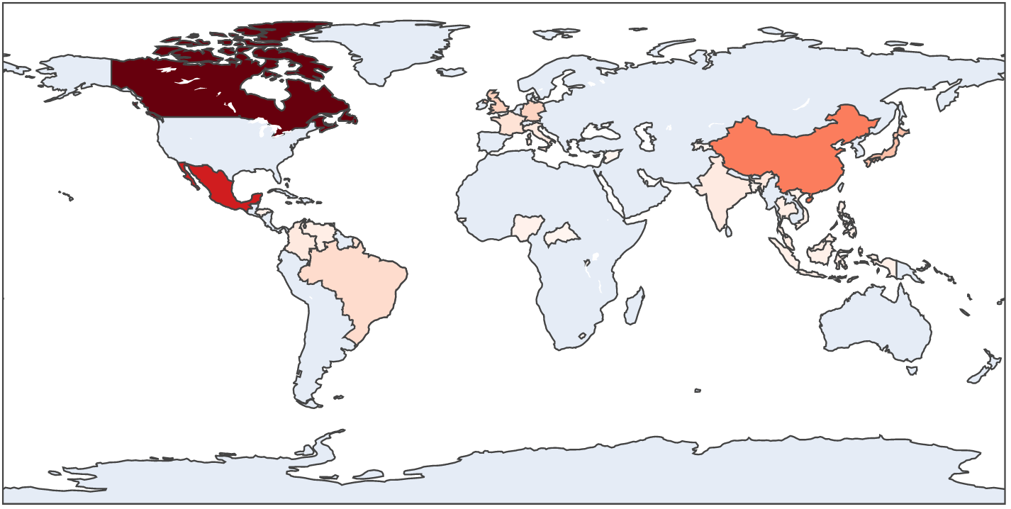
Let's plot only the export data:

from datatool import datatool
import numpy as np

def find_first_import_row(D):
    # COPY over your code from the previous exercise:

dt = datatool()

dt.load_csv('US_trade_2014_small.csv')

dt.sort_by_multiple_columns(['trade_direction','trade_volume'], [True, False])

D = dt.get_data_as_array()
first_import_row = find_first_import_row(D)

# Tell datatool to trim the rows from first_import_row onwards.
dt.use_n_rows(first_import_row)

# Color scale. More choices: https://plotly.com/python/builtin-colorscales/
dt.set_color_scale('reds')

# The choropleth_iso3() function uses a standard code for countries.
# The second parameter describes which column to use for heat-map
# like coloring. The third is what to show when the mouse hovers.
dt.choropleth_iso3('iso3', 'trade_volume', 'country')

dt.display()

3.73 Exercise: Type up the above in my_trade_analysis3.py, filling in the needed code. You should see something like:

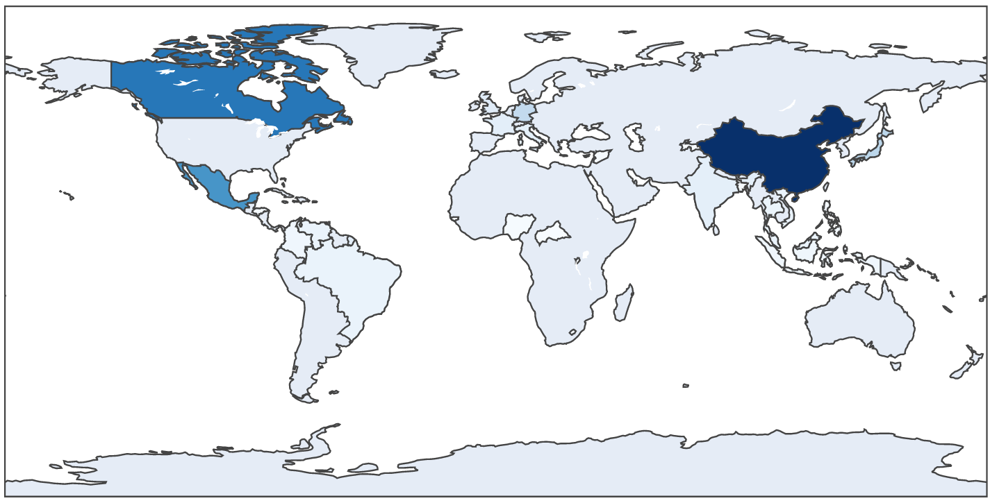
3.74 Exercise: In my_trade_analysis4.py, write code to display imports (and only imports). Change the color scale to 'blues'. You should get something like:

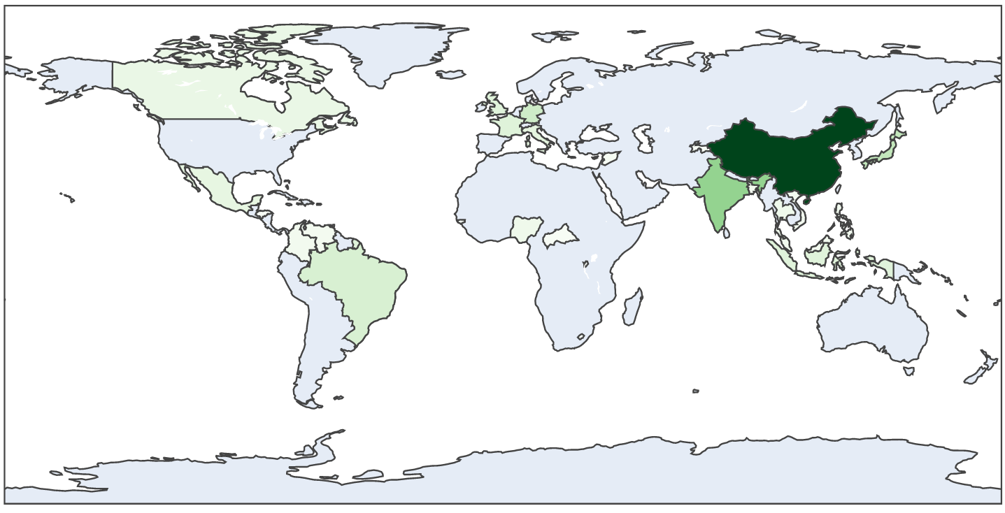
3.75 Exercise: Next, in my_trade_analysis5.py, modify the program in the previous exercise to print (using only the 'import' rows) plot a choropleth of sorted GDP, high to low.

3.76 Audio:

Now that we've seen plots of imports, exports and gdp ... what do these tell us?

In some ways, the trade volumes are no surprise. The large GDP countries generally show correspondingly large import-export volumes.
Most of what we see corresponds to conventional wisdom.
To get further insight or detect unusual patterns, we'd have to pore over these plots and write additional code to look ... what exactly?
Let's see what the gravity approach can do for us.

The gravity model of trade borrows an idea from physics:

The law of gravity says that the force of gravity between two objects (such as the earth and moon) is proportional to the product of their masses, and inversely proportional to the square of their distance.
We write this as: $$ F \;\; = \;\; G \frac{M_1 M_2}{r^2} $$ where $M_1$ and $M_2$ are the masses (think: weights) of the two objects, and $r$ is the distance between them. The number $G$ is a constant (typical in physics laws).
Using this idea, one can draw an analogy with trade between two countries (economic "objects"):
- One expects a high flow of trade between countries with large economic output (high GDP).
- But should distance matter? That is, should we get something like $$ \mbox{trade} \;\; = \;\; \frac{\mbox{GDP}_1 \mbox{GDP}_1}{\mbox{something}} $$
- The greater this "something", the less trade we should see.
To get a feel for this, let's calculate $$ \frac{\mbox{trade}}{\mbox{GDP}_1 \mbox{GDP}_1} $$ and see if that provides any insight.
The main purpose of the trade model is to compare what a formula might predict against actual trade flow (the sum of import and export trade volumes). Lower trade than expected could be for reasons of distance (high shipping costs), politics, or economic friction (difficult regulations, poor enforcement of local laws).

3.77 Exercise: Download US_trade_2014.csv and add code to my_gravity_analysis.py to complete a few supporting functions. Study the code to see how the ratio above is calculated from the data. The output expected is described in comments.

3.78 Audio:

3.79 Exercise: In the previous exercise, you applied the trade model to identify countries with high GDP with less than expected trade, resulting in a list of 7 countries. In your module pdf, explain why U.S. trade with these countries is lower than expected from the gravity model. For example, distance might explain why Australia is in the list. What about the others in the list?

Part B: the prisoner's dilemma

Start by reading this short article on the topic.

We'll begin with a few observations:

The prisoner's dilemma is a type of "game" that formalizes interactions between two players.
The formal study of such games is called game theory, an area of study that spreads across mathematics, economics and international negotiation.
The most fundamental kind of game is a two-player game in which each player simultaneously makes their move (as opposed to taking turns, as in chess).
In a one-shot game like the prisoner's dilemma, each player makes their move and that's the end of the game.
In an iterated version, there are multiple games in succession.
We will be interested in the iterated prisoner's dilemma
As you read in the article, the prisoner's dilemma game has many applications. It might not result in actual strategy, but often clarifies intentions and possibilities in a real-life scenario.

First, the rules of a one-shot prisoner's dilemma:

In our version (the most common one), a bank has been robbed and two robbery suspects (prisoners) are being separately interrogated.
If both stay silent, they can both get out and split the haul.
If both implicate the other, neither gets out.
If one implicates the other, and the other is silent, the implicator gets out and gets the whole haul.
In this formulation each prisoner must choose between two possible moves:
- Cooperate: "Cooperate" means to keep silent and not rat out the other prisoner.
- Defect: "Defect" means to rat out or implicate the other prisoner.
We'll use Prisoner-0 and Prisoner-1 to denote the two.
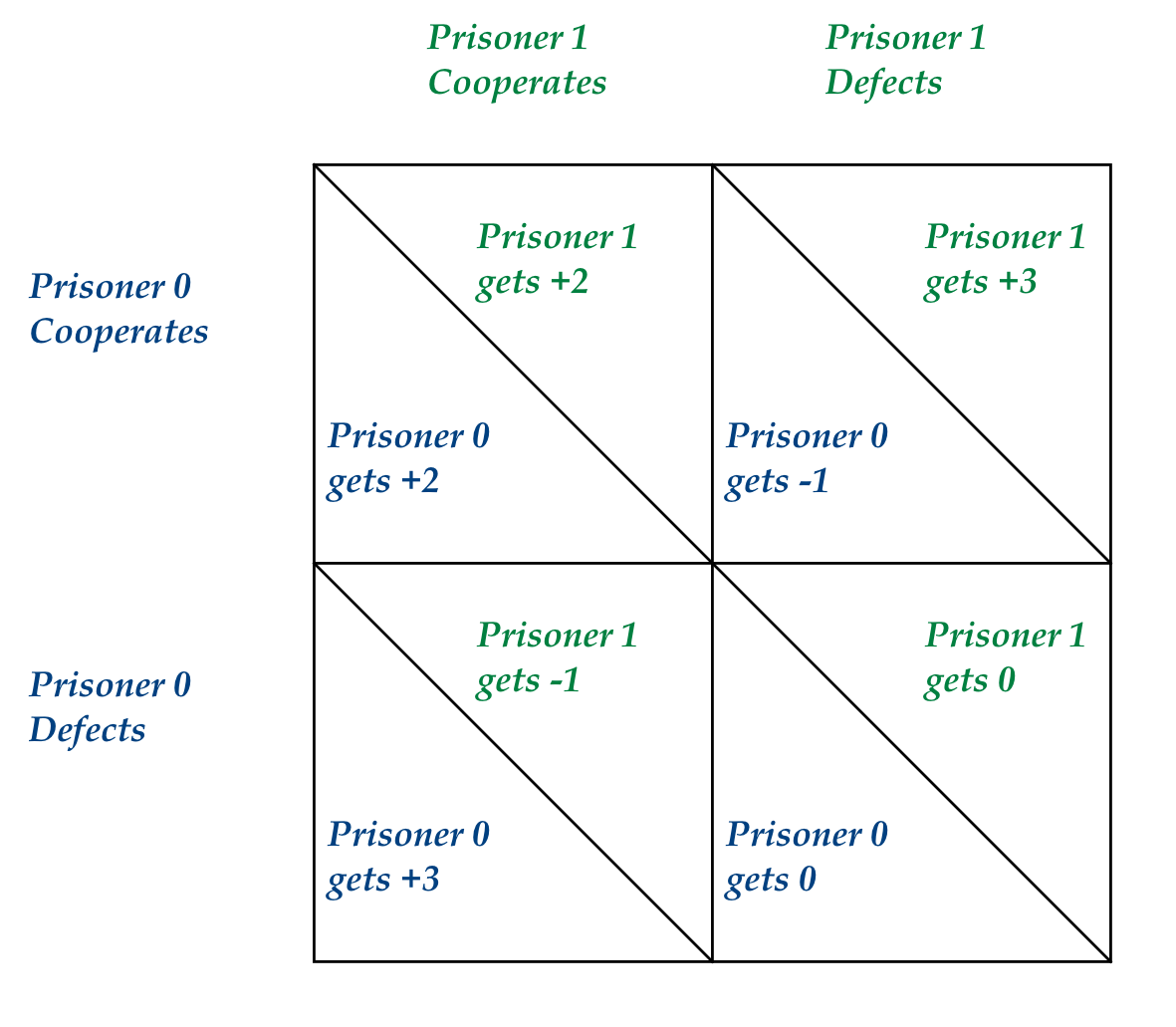
Thus, there are four possibilities, to which are associated four numeric outcomes (as points):
- Both cooperate, in which case both get 2 points (both split the haul of 4).
- Both defect, in which case both get 0 points.
- Prisoner-0 cooperates, Prisoner-1 defects:
  - Prisoner-0 gets -1 points (a penalty)
  - Prisoner-1 gets 3 points (the haul)
- Prisoner-0 defects, Prisoner-1 cooperates:
  - Prisoner-0 gets 3 points
  - Prisoner-1 gets -1 points
This is often expressed in a table:
Because we're going to simulate the playing of the game, we can play repeatedly with different strategies.
Our main goal: to evalute the average outcome for each strategy when played against other strategies.

The strategies we will evaluate

Strategy A: random. Simply pick randomly between "cooperate" and "defect".
Strategy B: tit-for-tat. Since this is a repeated game, each player can see what the other player did in the previous round. In tit-for-tat, a player uses the move made by the other player in the previous round.
Strategy C: randomized tit-for-tat. A variation of tit-for-tat that applies a little randomness (we'll see why).
Strategy D: gain-learning. This approach tries to learn from past games by slowly adjusting a parameter.
Strategy E: . You devise one.

Let's start with Strategy A.

3.80 Exercise: Download prisoner0.py, prisoner1.py, prisoner_game.py, and eval_strategyA.py. Examine the code in prisoner0.py to confirm that the implementation of strategy A is indeed to randomly choose between 'cooperate' and 'defect'. Then execute eval_strategyA.py to confirm this output. Increase the number of iterations to 10000 to see what the average turns out. (Change it back to 10 for submission.)

Clearly, one should be able to do better than random. Let's examine a strategy called tit-for-tat:

  If it's your first move, pick 'cooperate'
  Otherwise, play the same move your opponent picked in the last round.

The idea here is to extend the hand of cooperation (at first). As long as your opponent cooperates, you do too (in the next round). If your opponent defects, you do too in the next round.
In terms of coding, notice the parameters passed into a strategy:
```
def play_strategyA(my_moves, opponent_moves):
  
```
A player gets their own history of moves so far as a list, and their opponent's moves as a list.
Thus, the last element in the second list is the most recent move made by the opponent.
Although neither random nor tit-for-tat adjust their strategy with each round, the code is structured to allow that:
```
def update_strategyA(my_moves, opponent_moves, my_score):
  
```
Here, the two lists contain the moves played in the current round, and the score obtained for this player.
The idea with "update" is that one can adjust based on the latest score received (as we'll see below).

3.81 Exercise: Implement tit-for-tat in your prisoner0.py AND prisoner1.py. That is, write code to apply tit-for-tat in play_strategyB() in each of prisoner0.py and prisoner1.py files. Then, download and execute eval_strategyB.py. Then execute to confirm this output.

3.82 Exercise: Change the first part of Strategy-B in prisoner0.py to make the first move 'defect'. What do you observe as a result? Report in your module pdf.

We'll make two modifications to tit-for-tat to improve its robustness:

One problem is that it is too sensitive to the initial starting move of the opponent.
Another is that because it's so deterministic and rigid, tit-for-tat might get stuck in an endless pattern that might drive the result towards perpetually playing 'defect'.
Thus, the first modification is to make the first move random.
The second is occasionally make a random move, the frequency of which is governed by a parameter $\beta$ as follows:
- At each turn, with probability $\beta$, select a random move.
- Thus, if $\beta=0.1$ then for approximately 10% of the time, a random move will be selected.
- Think of $\beta$ as an "exploration" or "getting unstuck" move.
- At each turn, generate a random number between 0 and 1. If that number is less than $\beta$, pick randomly between 'cooperate' and 'defect'.
- The idea is, over many such trials, the fraction of such exploration moves will be $\beta$.
We'll call this randomized tit-for-tat and implement it as Strategy C.

3.83 Exercise: Implement randomized tit-for-tat by writing code in the play_strategyC() function in each of prisoner0.py and prisoner1.py files. Then, download and execute eval_strategyC.py. Then execute to confirm this output.

None of the strategies so far have adjusted "along the way" by learning from prior moves.

Let's now examine the possibility of learning from past moves (and outcomes of those moves):

Every program that plays games, such as chess-playing programs, learns by adjusting internal "strategy parameters".
Typically, such programs "train" by playing thousands of games and using outcomes to incrementally adjust the parameters.
Let's examine a highly simplified single-parameter version for Prisoner's Dilemma.
The parameter will be called $\alpha$ and the way $\alpha$ will be used to decide a particular move is:
- Choose 'cooperate' with probability $\alpha$.
- That is, generate a random number between 0 and 1. If the number lies between 0 and $\alpha$, pick 'cooperate'.
This part is easy. How should $\alpha$ be updated?
We will use the most recent outcome (the score) to update $\alpha$ as follows:
- If your last move was 'cooperate' and you received a positive score, then increment $\alpha$ slightly.
- If your last move was 'defect' and you received a negative score, then increment $\alpha$ slightly.
- In all other cases, decrement $\alpha$.
Remember that $\alpha$ is the probability of choosing 'cooperate' so if 'defect' did badly (negative) then we need to increase $\alpha$.
We'll call this strategy gain-learning and implement it in Strategy-D.

3.84 Exercise: Implement gain-learning by writing code in the update_strategyD() function in each of prisoner0.py and prisoner1.py files. Note that to increment or decrement alpha, just call incr_alpha() or decr_alpha() respectively. Download and execute eval_strategyD.py. Then execute to confirm this output. In your module pdf, explain the reason for the if-statement in each of the increment/decrement functions.

3.85 Audio:

Now, let's play the strategies against each other.

3.86 Exercise: Download and execute eval_ABCD.py. Then execute to confirm this output. Clearly, we see a small benefit to adjusting the strategy as we go.

Now it's your turn.

3.87 Exercise: In your prisoner0.py and prisoner1.py, implement your own strategy as Strategy-E. Then download and execute eval_all.py to evaluate. Report your results in your module pdf, explaining your strategy and providing an intuition for its performance.

About the Prisoner's Dilemma and game theory:

There is an interesting history to Prisoner's Dilemma:
- A few international competitions were held to allow various competitors to submit strategies in code for the iterated game.
- Some were quite complex, with hundreds of lines of code.
- Surprisingly, tit-for-tat turned out to be one of the best performers.
- One can create an evolutionary version of the iterated game where successive rounds result in knocking out losing strategies.
- Tit-for-tat wins often enough that this has sometimes been interpreted to describe how cooperation evolved in human and animal social groups.
Game theory is an interesting subfield of economics and international affairs (including military strategy).
- Variations include N-player games, games with random outcomes, games with coalitions, and other such rules.
- It is generally a highly mathematical field, with analyses of all kinds of games and strategies.
- At the same time, it's generally easy to write up games and strategies in code to simulate and evaluate.
- The type of game theory we've examined is quite different from the algorithmic approach used in devising chess-playing programs.

Optional further exploration

If you'd like to explore further:

Try this this TED talk about how the rules of international trade have changed.
A book (movie) worth reading (watching) about one of the key contributors to game theory, John Nash: A Beautiful Mind.
Try this TED talk on an interesting take on the Prisoner's Dilemma.

Back to Module 3