The goal of this module is to introduce the
all important feature called arrays, of central
importance in working with numeric data.
0.0 Audio:
0.0 First, a list of lists
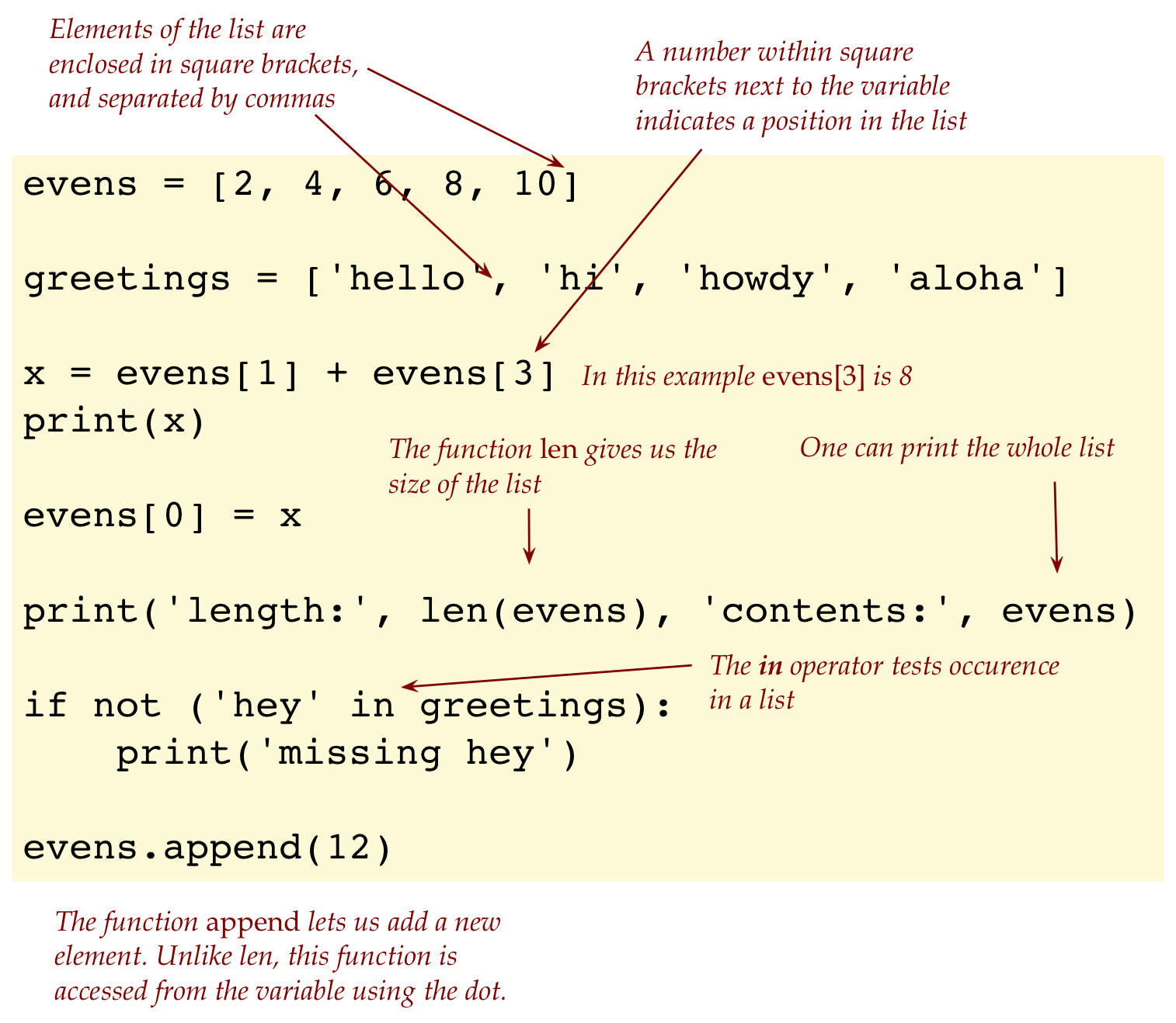
Recall a basic list:
# A list of numbers:
evens = [2, 4, 6, 8, 10]

# A list of strings:
greetings = ['hello', 'hi', 'howdy', 'aloha']

# Access list elements using square brackets and index
x = evens[1] + evens[3]
print(x)

# We can change the value at an individual position
evens[0] = x

# Recall: len() gives us the length of the list
print('length:', len(evens), 'contents:', evens)

# Example of using in to search inside a list:
if (not 'hey' in greetings):
    print('missing hey')

# Add something new to the end of a list
evens.append(12)

# Write code here to increment each element by 2

print(evens)
# Should print: [12, 4, 6, 8, 10, 12]
0.1 Exercise:
First, in
my_list_example.py,
type up the above to see what it prints (without including the
missing code). Then, in
my_list_example2.py,
add the missing code to increment each list element by 2.
Let's recall a few things we learned about lists via this example:
Why are lists useful?
The real power comes from being able to use a loop to
Create elements, as in:
    for i in range(1, 10, 2):
        A.append(2*i)
Perform some action on each element, as in:
    for i in range(len(A)):
        A[i] = 2 * A[i]
And one can use multiple lists as well, as in:
    for i in range(len(A)):
        B[i] = A[i] + 5
Lists allow both index iteration as above but also
content iteration:
    total = 0
    for k in A:
        total = total + k
As it turns out, we can make a list of lists.
That is, a list whose elements are themselves lists.
For example:
A = [ [2,4,6,8,10], [1,3,5,7,9] ]

x = A[1]          # The 2nd element is a list
print(x)          # Prints [1,3,5,7,9]

y = A[1][3]       # 4-element of 2nd list
print(y)          # 7

print(len(A))     # 2
print(len(A[0]))  # 5
Note:
The inner square brackets are used for the two lists
contained in the one larger list:
A = [ [2,4,6,8,10], [1,3,5,7,9] ]
And the outermost square brackets indicate the single list
with two items:
A = [ [2,4,6,8,10], [1,3,5,7,9] ]
A[1] refers to the 2nd element of the whole thing, which
means A[1] is the 2nd inner list:
A = [ [2,4,6,8,10],[1,3,5,7,9]]
x = A[1] # The 2nd element is a list
print(x) # Prints [1,3,5,7,9]
Since A[1] is a list itself, we can access its elements
using an additional set of square brackets:
A = [ [2,4,6,8,10],[1,3,5,7,9] ]

y = A[1][3]       # 4-element of 2nd list
print(y)          # 7
And the len() function applied to the whole list will give
2, while applying it to one of the constituent lists will give that
list's length:
print(len(A))     # 2
print(len(A[0]))  # 5
0.2 Exercise:
Consider the following code:
A = [[1,2,3,4], [4,5,6,7], [8,9,10,11,12]]
x = A[?][?]
print(x)     # Should print 7

# Write code to increment every element using a nested for-loop:


print(A)
# Output should be: [2, 3, 4, 5], [5, 6, 7, 8], [9, 10, 11, 12, 13]]
In
my_list_example3.py,
add the right numbers to replace the question marks. Then, write a
nested for-loop to increment every element of every constituent list.
0.3 Audio:
Can one make a list of lists of lists?
Think of a single list as one dimensional:
A = [2, 4, 6, 8, 10]
print(A[3])
In a one-dimensional list, we need a single number to access a data
value in the list:
print(A[3])
And a list of lists as two dimensional:
A = [ [2,4,6,8,10], [1,3,5,7,9] ]
print(A[0][2])
In a two-dimensional list, we need two numbers to access a data
value in the list:
print(A[0][2])
Think of a list of lists of lists
as three-dimensional, which means three numbers fix the
position of a element.
For example:
A = [ [ [1,2], [3,4], [5,6] ], [ [7,8], [9,10], [11,12] ] ]

print(A[0][2][1])     # Prints 6
It's a bit hard to see the list of lists of lists:
First, there's the outermost list with two elements:
Get the this list's 3rd element A[0][2] (this produces a list)
Get this last list's 2nd element A[0][2][1].
0.1 Arrays: a more efficient type of list
While lists are useful and easy to use, they are a bit inefficient
"under the hood":
Very large lists (million elements and higher) can slow down a program.
And a list-of-lists is even slower for large sizes, and
takes up unneccessary extra space (compared to arrays).
Some of the most compelling uses involve the array
equivalent of a list-of-lists-of-lists: an image.
As we will see, a regular color image will turn out
to be a three dimensional array while a black-and-white
image will turn out to be a two-dimensional array.
About arrays:
Arrays were created as a separate structure in Python to enable
efficient processing of lists of numbers, especially
multidimensional lists.
Because arrays are in a separate part of Python, the syntax
around arrays is a bit different, for example:
A = np.array([1,2,3,4])
Arrays constitute a large topic in Python, and its
advanced features can be fairly complex.
Our goal here is only a light introduction so that we
can work with images.
Let's start with an example of
a single dimensional array, the cousin of a plain list:
import numpy as np

A = np.array([1,2,3,4])

print(type(A))             # What does this print?
A[1] = 5                   # Replace 2nd element
print(A)                   # [1 5 3 4]
print(A.shape[0])          # 4
print('len(A)=',len(A))    # 4

# A[4] = 9
# A.append(9)
0.4 Exercise:
Type up the above in
my_array_example.py.
Try un-commenting in turn each of the two commented-out lines
at the end, and report the errors in your module pdf.
(Restore your program by commenting out both.)
Let's point out a few things:
To gain efficiency, arrays trade away some flexibility and ease
of use.
For example, we now need to import this special package
called
numpy:
import numpy as np
Once we do this, the syntax for making an array with actual
data is, as we've seen:
A = np.array([1,2,3,4])
A brief aside on the Python keyword as:
We use as to create shortcuts.
We could write code like this:
import numpy
A = numpy.array([1,2,3,4])
The as keyword lets us create a short form.
We could have made it even shorter:
import numpy as n
A = n.array([1,2,3,4])
but this is frowned up on Python culture.
Over time, a sort-of convention about naming has taken place
in Pythonworld.
Which is why you'll see all example code using
numpy as np.
End of digression.
Notice that that actual data is fed into
numpy'sarray
function as a list:
import numpy as np
A = np.array( [1,2,3,4] )
The actual array so created is in fact in the variable
A.
To work with elements in the array, we use square brackets
with the variable
A:
A[1] = 5 # Replace 2nd element
The standard function
len()
works as we expect:
print('len(A)=',len(A))
However, the array has a feature that is more general called
shape:
print(A.shape[0]) # 4
At first this seems cumbersome, and for single-dimensional
arrays, it is.
But for multiple dimensions, it's convenient to have
the length of each dimension handy.
This is what
shape
has.
shape[0]
has the first dimension (the length of the array along the first dimension).
shape[1]
has the length along the second-dimension, and so on.
Of course, for a single dimensional array, there's only
shape[0].
One of the efficiency tradeoffs is that an array has
a fixed size. Which means, to add a new element, we have to
rebuild the array.
Thus, to add an element in the above example, we need to write:
A = np.append(A, 9)
print(A)        # [1 5 3 4 9]
This creates a new array with the added element.
Typically most scientific applications do not change
sizes on the fly, and so, this is not a serious restriction.
Numpy has powerful features that simplify manipulation
of numeric arrays.
For example, consider:
import numpy as np

A = np.array([1, 2, 3])
B = np.array([4, 5, 6])

C = A + B            # Direct element-by-element addition
print(C)             # [5, 7, 9]

D = np.add(A, B)     # The same, via the add() function in numpy
print(D)             # [5, 7, 9]

E = B - A            # Elementwise subtraction
print(E)             # [3, 3, 3]
0.5 Exercise:
Type up the above in
my_array_example2.py
and add a line that multiplies the arrays
A
and
B
element-by-element, and prints the result
([ 4 10 18]).
0.6 Exercise:
In
my_list_version.py,
let's remind ourselves about how lists work. Start by
examining what happens with:
X = [1, 2, 3]
Y = [4, 5, 6]
Z = X + Y
print(Z)          # What does this print?

# Write code here to compute Z as element-by-element addition
# of X and Y (to give [5, 7, 9])

print(Z)
Then add code to perform element-by-element addition.
Numpy also has a number of functions that act on arrays
and return arrays, for example:
One can apply a function like square-root element-by-element:
A = np.array( [1, 4, 9, 16] )
B = np.sqrt(A)
print(B)        # [1. 2. 3. 4.]
One of the most convenient is to have Numpy create an
array with random elements, as in:
# Roll a die 20 times
A = np.random.randint(1, 7, size=20)
This produces an array of size 20 with each element randomly
chosen from among the numbers 1,2,3,4,5,6.
Numpy has its own random-generation tool:
np.random
This has a function
randint()
that takes the desired range (inclusive of first, excluding
last), and the desired size of the array.
One can also test membership using the in operator:
For example, suppose we roll a die 20 times and want
to know whether a 6 occured:
# Roll a die 20 times
A = np.random.randint(1, 7, size=20)
if 6 in A:
    print('Yes, there was a 6')
0.7 Exercise:
In
my_dice_problem.py
fill in code below to estimate the chances that you get a
total of 7 at least once when rolling a pair of dice 10 times.
successes = 0
num_trials = 1000
for n in range(num_trials):
    # Fill your code here

print( successes/num_trials )
To do so, generate one array called A of length 10 with random
numbers representing one die (selected from 1 through 6).
Then
generate a second array called B that represents the 10 rolls of
the second die. A success occurs when A[i]+B[i] is 7 for
some i. Can you solve this without actually accessing the i-th
element in a loop?
0.8 Audio:
0.2 2D arrays
Here, 2D is short for two-dimensional.
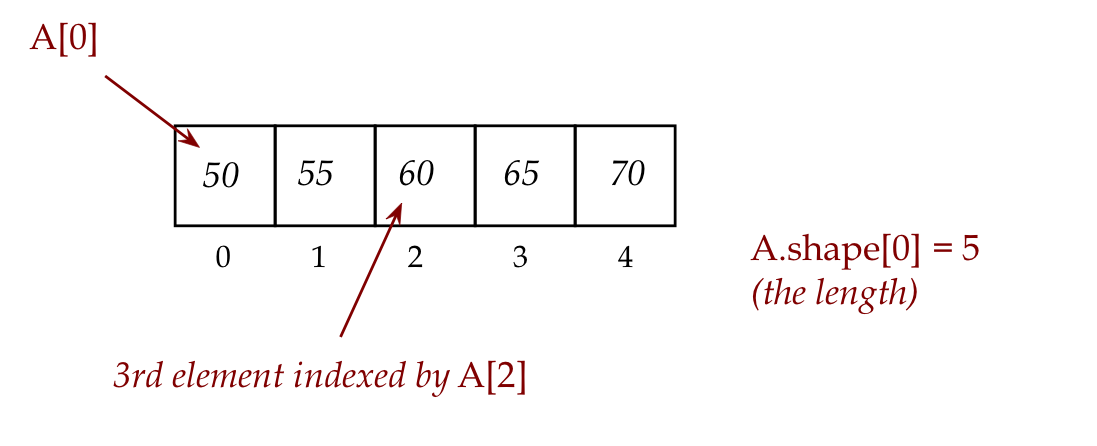
Let's begin with a conceptual depiction of a 1D
(one-dimensional) array:
First, suppose we create an array of 5 numbers as in:
A = np.array([50, 55, 60, 65, 70])
A convenient way to visualize this is to draw these numbers
in a series of adjacent "boxes" as in:
Because we need a way to use our keyboard to enter elements,
we use a particular kind of syntax, comma-separation with
square-brackets to specify the elements.
We use a similar type of syntax to access a particular
element in this array, as in:
print(A[2])
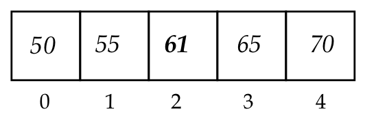
We can also change an element in an array:
A[2] = 61
which will result in the visualization
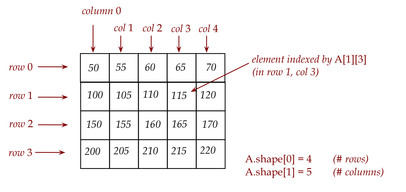
To explain how a 2D array works, let's start with its
conceptual visualization, via an example:
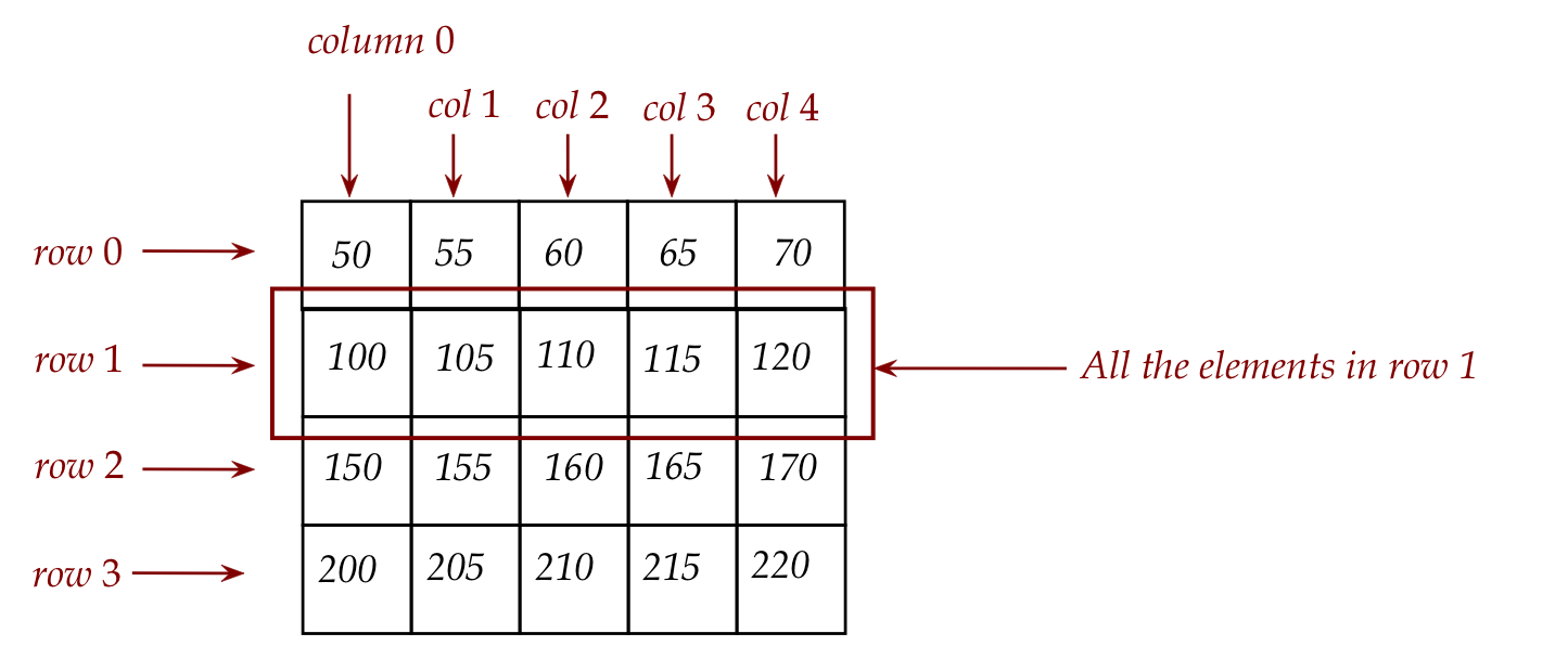
Consider this visualization of a 2D array:
We use the term row to describe the contents
going across one of the series of boxes going left to right:
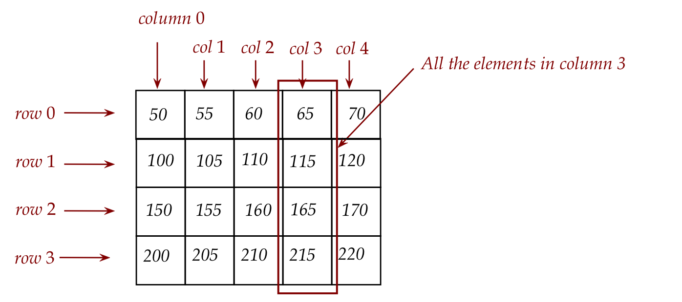
And the term column (shortened to col in
our pictures) to describe the series of boxes going vertically top
to bottom:
Observe:
The number of elements in a row is the number of columns.
The number of elements in a column is the number of rows.
Again, because our limited keyboard doesn't let us draw
boxes, we need a way to type in a 2D array. We do so by writing out
a 2D array as a series of comma-separated rows:
Here, we've added whitespace (that's allowed) to line up the rows
so that it's as close to our visual understanding as possible.
To access a particular element, we need the row number and
column number, as in:
print(A[1,3]) # NOT A[1][3]
Important: Unlike a list-of-lists,
arrays use comma separation and not
box-separation. For comparison:
# List of lists:
X = [ [2,4,6,8,10], [1,3,5,7,9] ]
print(X[0][2])
# 2D array:
X = np.array([ [2,4,6,8,10], [1,3,5,7,9] ])
print(X[0,2])
Unfortunately, arrays allow box-separation as well (for access) but
this causes problems in other array operations (slicing): so
please use comma-separation with a single set of square brackets
for arrays.
Just as we used a for-loop for a single array, it is very typical
to use a nested for-loop for a 2D array:
For comparison, let's look at a 1D array:
A = np.array( [1, 4, 9, 16] )
for i in range(A.shape[0]): # Recall: A.shape[0] is the size
print(A[i])
The equivalent for a 2D array is:
A = np.array([ [50,   55,  60,  65,  70],
               [100, 105, 110, 120, 125],
               [150, 155, 160, 165, 170],
               [200, 205, 210, 215, 220] ])
for i in range(A.shape[0]): # number of rows
for j in range(A.shape[1]): # number of columns
print(A[i,j])
To make the code a bit more readable, we could write
num_rows = A.shape[0]
num_cols = A.shape[1]
for i in range(num_rows):
    for j in range(num_cols):
        print(A[i,j])
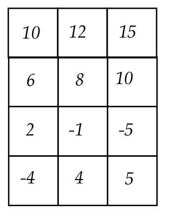
0.9 Exercise:
Consider this conceptual 2D array:
In
my_2D_array.py,
write code to create the array, and then a nested loop to print
the array so that the output has one row on each line, with whitespace
between elements, as in:
10  12  15
6  8  10
2  -1  -5
-4  4  5
0.10 Exercise:
In
my_2D_array2.py,
use the same array above and structure a nested loop to
compute the sum of elements down each column so that the output is:
Column 0 total is 14
Column 1 total is 23
Column 2 total is 25
0.11 Audio:
About 2D arrays:
Although our examples show arrays of integers, the Numpy
package supports a wide variety of data types, including floats,
chars, strings and such.
There are even specially "compacted" versions of integers
to enable working with extremely large arrays.
There are two common (and quite different) uses of 2D
arrays:
One is for a mathematical construct called a matrix,
which you'd learn in a course called linear algebra.
The other is for images, which we'll look at next.
0.3 A greyscale image is really a 2D array of integers
0.12 Exercise:
Type up the above in
my_image_example.py
and download
drawtool.py
into the same folder.
When you run and see the result on your laptop, see if you can
position yourself 10 feet away from your laptop so that your
eyes don't see the faint lines that outline the grid.
What is a greyscale image?
By greyscale, we mean black-and-white (no colors)
but more specifically (and typically) 256 shades of grey.
Consider this illustration showing an image on the left
with a small part of it zoomed in:
Any digital image is really a 2D arrangement of small squares
called pixels, in rows and columns (just like an array).
In a greyscale image, each pixel is colored a shade of grey.
In standard greyscale images, there are 256 shades of grey
numbered 0 through 255 where 0 is black, and 255 is white.
Now let's go back to the code and examine what we wrote:
The first number (50) is a shade of dark grey (almost black).
The next number (55) along that row specifies a slightly
lighter (but still quite dark) shade of grey.
Now consider 200, the first number in the 4th row: this is a
shade of light grey, while 220 at the end is nearly white.
Thus, a greyscale image is nothing but a 2D array of
integers whose values range between 0 and 255 (inclusive).
Our eyes are fooled into seeing a seamless image because
of high resolution. Whereas our eye can see the individual pixels
in the example above, a regular image has thousands of pixels,
which is enough to fool the eye.
In a color image, as we will later see, we'll need three
numbers for each pixel (the amounts of red, green, blue).
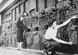
About the greyscale machine pictured above:
This is an image of the ACE computer, one of the world's
earliest computers, designed by none other than Alan Turing,
computer science pioneer and WWII hero.
To give you a sense of how primitive these were, your laptop
with 8GB RAM has more than 60 million times the memory of the ACE.
And yet, the ACE was a landmark technological wonder at its time.
0.13 Exercise:
In
my_image_example2.py,
create a 10 x 12 (10 rows, 12 columns) greyscale image
that is intended to be the logo of a fictitious company.
In your module pdf, include a screenshot of the image,
the name of the company, and what the company does.
Points for humor and creativity. We'll post the best ones.
Let's now work with an actual image:
from drawtool import DrawTool
import numpy as np
dt = DrawTool()
dt.set_XY_range(0,10, 0,10)
dt.set_aspect('equal')
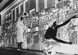
greypixels = dt.read_greyimagefile('eniac.jpg')
# greypixels is a 2D array
dt.set_axes_off()
dt.draw_greyimage(greypixels)
dt.display()
# Add code to print the number of rows, number of columns
# Should print: rows = 189 columns = 267
0.14 Exercise:
Type up the above in
my_image_example3.py
and download eniac.jpg.
Add code to print the number of rows and number of columns,
then in your module pdf, report these numbers. Also, spend 15 minutes
learning about the ENIAC, its inventors,
its significance, and write a short paragraph about this in your pdf.
Image formats:
When an image is stored as a file, the file needs to contain
all the integers that comprise the 2D array (for greyscale images)>
Large images can take quite a bit of space. For example,
a 1000-row x 1000-column image will have one million pixels.
Yet many images have vast expanses of the same color or
intensity and they offer a chance to compress (use less
space by being clever).
Image formats arose as a result of wanting to both compress
the storage and to store meta-info about images.
Popular formats include: JPG, PNG, TIFF and Bitmap.
Typically the last part of the filename (the ".jpg" in
"eniac.jpg") tells you the format.
Python provides a way of reading from these formats so that
we don't have to worry about the details.
Let's now modify a greyscale image:
from drawtool import DrawTool
import numpy as np

dt = DrawTool()
dt.set_XY_range(0,10, 0,10)
dt.set_aspect('equal')

greypixels = dt.read_greyimagefile('eniac.jpg')

greypixels2 = np.copy(greypixels)
num_rows = greypixels2.shape[0]
num_cols = greypixels2.shape[1]

lightness_factor = 10

for i in range(num_rows):
    for j in range(num_cols):
        value = greypixels[i,j] + lightness_factor
        if value > 255:
            value = 255
        greypixels2[i,j] = value

dt.set_axes_off()
dt.draw_greyimage(greypixels2)

# To save an image, use the save_greyimage() function:
# dt.save_greyimage(greypixels2,'eniac-light.jpg')

dt.display()
0.15 Exercise:
Type up the above in
my_image_example4.py
and try different values (in the range 10 to 100) of the
lightness_factor.
In your module pdf, explain the purpose of of the
if-statement inside the loop.
0.16 Exercise:
In
my_image_example5.py
write code to create the "photo negative" of a greyscale
image (black turns to white, white to black, light grey to dark grey,
dark grey to light grey, and so on). For example, applying this
to the eniac.jpg image should result in
eniac-negative.jpg.
0.17 Audio:
0.4 A color image is a 3D array of integers
About color images:
In a color image, each pixel will have a color instead of a "greyness"
factor.
Unfortunately, one cannot easily represent colors with a single
number.
There are many ways of using multiple numbers to encode
colors.
We'll use the most popular one: specify the strengths of the
three primary colors (Red, Green, Blue).
This approach is so popular that we refer to it simply as RGB.
The "amount" of red is a number between 0 and 255, the
amount of green is another such number, as is the amount of green.
Thus, each color is a triple of numbers, for example:
(255,0,0) is all red (no green, no blue)
(0,255,0) is all green (no red, no blue)
(0,0,255) is all blue (no red, no green)
Let's try a few more:
(255,255,0)
(100,255,255)
(200,200,200)
(grey is R,G,B all equal)
(0,0,0)
(255,255,255) is white
When each pixel needs three numbers and there's a grid of pixels,
how do we store the numbers?
We use a small array (of size 3) to store the triple.
Then each pixel in the 2D array of pixels will have
an array of size 3.
0.18 Exercise:
Type up the above in
my_color_example.py.
Then in
my_color_example2.py,
go back to your greyscale logo from earlier and design a better 10 x 12 color
logo for the same company. Put these side by side in your module pdf.
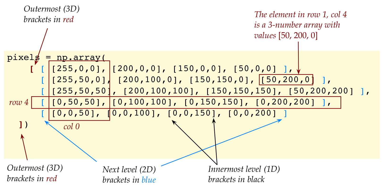
Let's point out the structure inherent in the above 3D array:
Next, let's work with actual color images with an example application:
converting color to greyscale:
from drawtool import DrawTool
import numpy as np
dt = DrawTool()
dt.set_XY_range(0,10, 0,10)
dt.set_aspect('equal')
# The image file is expected to be in the same folder
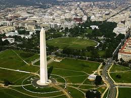
pixels = dt.read_imagefile('washdc.jpg')
num_rows = pixels.shape[0]
num_cols = pixels.shape[1]
greypixels = dt.make_greypixel_array(num_rows, num_cols)
for i in range(num_rows):
for j in range(num_cols):
# Average of red/green/blue
avg_rgb = (pixels[i,j,0] + pixels[i,j,1] + pixels[i,j,2]) / 3
# Convert to int
value = int(avg_rgb)
greypixels[i,j] = value
dt.set_axes_off()
dt.draw_greyimage(greypixels)
# Notice: saving to a different image format (PNG):
dt.save_greyimage(greypixels, 'washdc-grey.png')
dt.display()
0.19 Exercise:
Type up the above in
my_color_example3.py
and download
washdc.jpg.
What is the file size of the original versus the new greyscale one?
Read further about JPG vs PNG and in your module pdf,
explain why the PNG format needs more storage space than the JPG format.
Next, consider the following program:
from drawtool import DrawTool
import numpy as np

dt = DrawTool()
dt.set_XY_range(0,10, 0,10)
dt.set_aspect('equal')

pixels = dt.read_imagefile('washdc.jpg')

num_rows = pixels.shape[0]
num_cols = pixels.shape[1]

for i in range(num_rows):
    for j in range(num_cols):
        if ( (pixels[i,j,1] > pixels[i,j,0])
             and (pixels[i,j,2] < 0.5*pixels[i,j,1]) ):
            pixels[i,j,0] = 0
            pixels[i,j,1] = 0
            pixels[i,j,2] = 255

dt.set_axes_off()
dt.draw_image(pixels)

dt.display()
0.20 Exercise:
Type up the above in
my_color_example4.py.
You already have
washdc.jpg.
What did we just do?
We are examining the R,G,B values for each pixel, to
see if the condition (G > R) and (B < G) is satisfied.
When the condition is satisfied, we are overwriting
the pixel with a new (all blue) color.
What we're trying to do is identify greenery
by asking: when do we have the Green value a bit larger
than the Red value and much larger than the Blue value?
Why is this useful? This is essentially what many
satellite-image applications do: identify areas of interest
for urban planning, crop surveys,
environmental assessment (think: rainforest), and so on.
Notice that this rule does not capture all greenery.
0.21 Exercise:
In
my_color_example5.py,
try to add additional rules to capture the remaining greenery (the
trees) and set those pixels to blue as well. Show the result in
your module pdf.
0.22 Audio:
0.5 Arrays and slicing
Slicing can be applied to arrays in the same way that we
used them earlier for lists with one major difference, as
we'll point out.
For example:
import numpy as np

print('list slicing')
A = [1, 4, 9, 16, 25, 36]
B = A[1:3]                 # B has [4, 9]
print(B)
B[0] = 5                   # B now has [5, 9]
print(B)
print(A)                   # What does this print?

print('array slicing')
A = np.array( [1, 4, 9, 16, 25, 36] )
B = A[1:3]                 # B "sees" [4, 9]
print(B)
B[0] = 5                   # What happens now?
print(B)
print(A)                   # What does this print?
0.23 Exercise:
Type up the above in
my_slicing_example.py
and report the results in your module pdf.
Let's explain:
The slicing expression
1:3
in
A[1:3]
refers to all the elements from position 1 (inclusive)
to just before position 3 (so, not including position 3).
With lists, a new list is created with these elements:
A = [1, 4, 9, 16, 25, 36]
B = A[1:3]
So, writing into the new list (B) does not affect the old
list (A) from which the slice was taken.
But with arrays, a slice is only a view as if
we were giving a name to a zoomed-in-part:
A = np.array( [1, 4, 9, 16, 25, 36] )
B = A[1:3]
Here, array B refers to the segment (that's still in A)
from positions 1 to 2.
This is why, if you make a change to B, you are actually
changing A.
Why did they do this?
The reason is, many image processing applications require
working on parts of images.
Then, with regular slicing, if we were to pull out parts
and modify them, we'd have to write them back in.
Slicing makes it convenient to write directly into parts of images.
Slicing is a big sub-topic so we'll just point out a few useful things
to remember via an example:
# Color image:
A = np.array(
    [ [ [255,0,0], [200,0,0], [150,0,0], [50,0,0] ],
      [ [255,50,0], [200,100,0], [150,150,0], [50,200,0] ],
      [ [255,50,50], [200,100,100], [150,150,150], [50,200,200] ],
      [ [0,50,50], [0,100,100], [0,150,150], [0,200,200] ],
      [ [0,0,50], [0,0,100], [0,0,150], [0,0,200] ]
  ])

B = A[4:5,:,: ]   # The last row
print(B)
C = A[:,1:2,:]    # The second column
print(C)
D = A[:3,:2,:]    # The pixels in rows 0-2 and cols 0-1
print(D)
Note:
A different slice can be specified for each dimension of
a multidimensional array.
When neither end of a slicing range is specified, that implies
all the elements, as in:
B = A[4:5, :,: ] # The last row
Here, the stand-alone colons imply the whole range for the
2nd and 3rd array index positions.
It is possible to specify just one limit as in:
D = A[:3, :2,:] # The pixels in rows 0-2 and cols 0-1 <
In the first (row) case, we're saying "all rows from the start up to
row 2".
Let's apply slicing to creating a cropped image:
from drawtool import DrawTool
import numpy as np

dt = DrawTool()
dt.set_XY_range(0,10, 0,10)
dt.set_aspect('equal')

pixels = dt.read_imagefile('washdc.jpg')

# Crop from row 50 to 179, and column 50 to 199
pixels2 = pixels[50:180, 50:200]

dt.set_axes_off()
dt.draw_image(pixels2)

dt.display()
0.24 Exercise:
In
my_slicing_example2.py
change the cropping so that the Washington Monument shows up
centered in your cropped image, with little else around it.
Include your cropped image in your module pdf.