Enhance your understanding of how to use def to write functions, then invoke them.
Write code with function definitions and invocations.
Write and debug code with functions
Explore the different ways in which parameters work.
Identify new syntactic elements related to the above.
2.0 Audio:
2.0 Wait, stop!
Before continuing it is essential to review functions as
described in Module 2 of
Unit-0
What to review most carefully:
The notion of how execution starts outside a function, goes
into a function, and comes back to where the function was invoked.
Important: When we come back to where the function
was invoked, we continue execution just after the invocation.
2.1 Exercise:
Please review that module. Now.
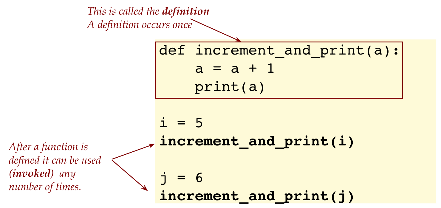
2.1 A simple example
Consider this program:
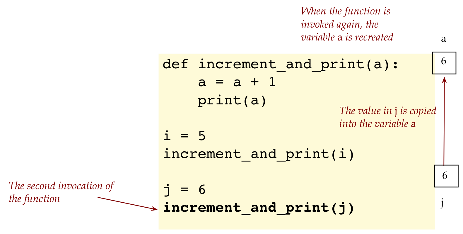
def increment_and_print(a):
    a = a + 1
    print(a)

i = 5
increment_and_print(i)

j = 6
increment_and_print(j)
2.2 Exercise:
Type up the above in
my_func_example.py
Then, just before the j=6 statement, print the value of i.
Let's explain:
Let's start by distinguishing between a function
definition (which merely tells Python what the function is
about), and invocation (which asks Python to execute the
function at that moment):
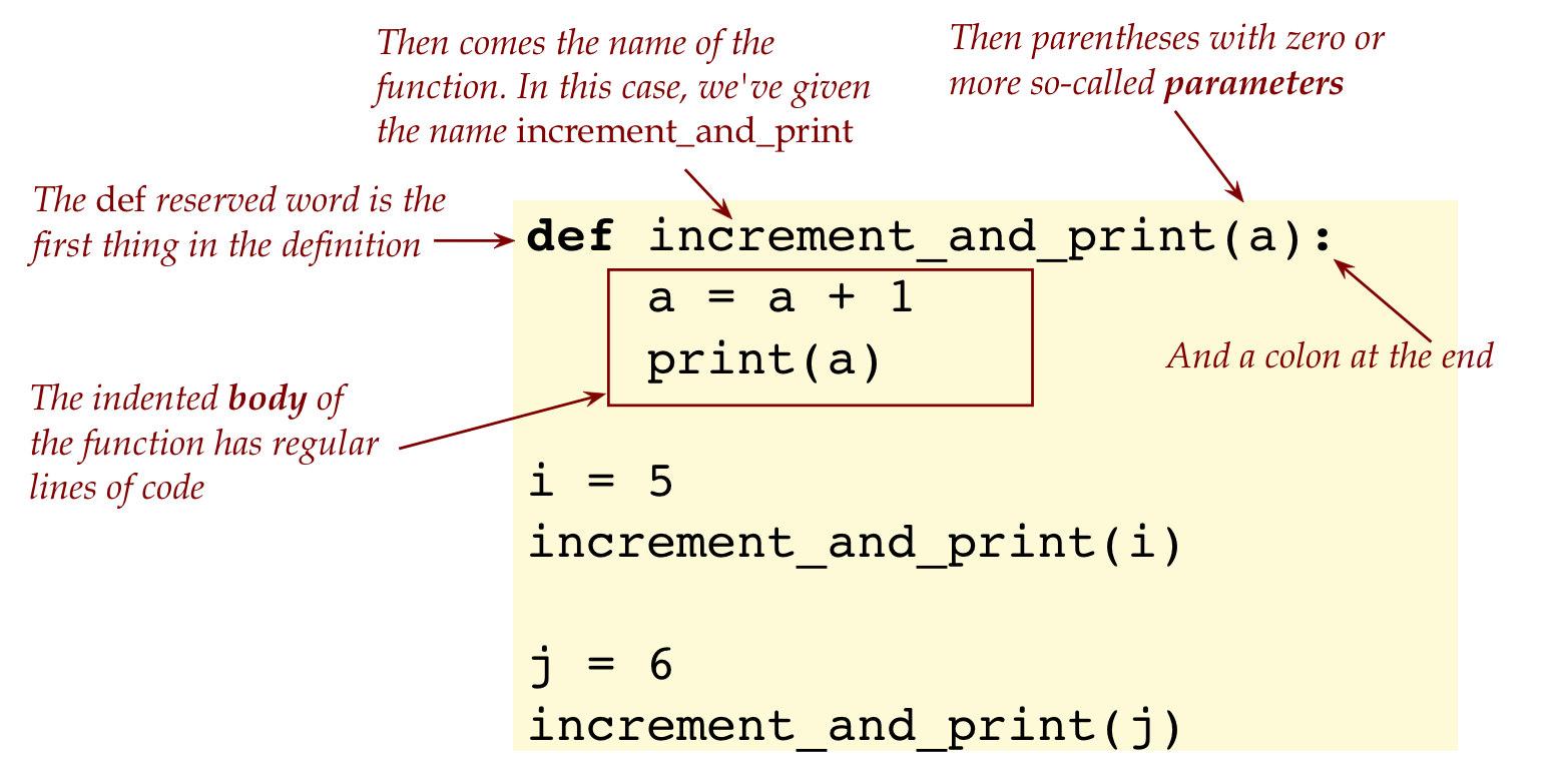
Now let's peer into what constitutes a definition:
In the above case, the function
increment_and_print
has only one parameter called
a.
In the future, we'll see that a function can have
several parameters, separated by commas.
For example
def increment_and_print(a, b, c):
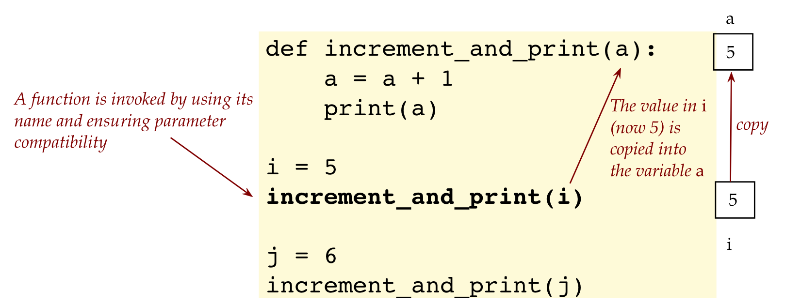
Next, let's examine how execution proceeds, starting
with what happens when a function is invoked:
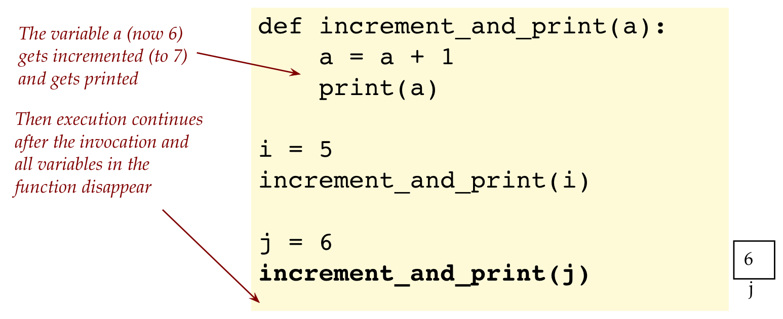
Once execution is inside the function:
Next, execution moves further into the second invocation:
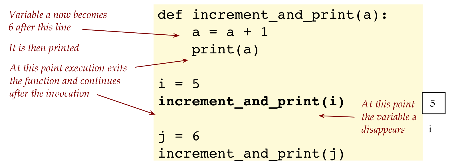
The code inside the function now executes (again):
Important: Did you notice that neither
i
nor
j
was affected by the incrementing of
a?
This is because the value in
i
was copied into the freshly-created
a
at the moment the function was invoked.
Even though
a
got incremented, that did not affect
i.
Variables like
a
that appear in the parentheses of a function definition
are called parameters.
What does a function do with its parameters?
Think of the parameters as variables that can be used
as regular variables for any purpose.
For example, consider this program:
def print_from_one_to(a):
    print('Printing between 1 and ', a)
    for i in range(1, a+1):
        print(i)

print_from_one_to(5)
print_from_one_to(6)
Here, we used the parameter
a
in setting the upper limit of a for-loop.
Important: When a function is defined with a
parameter, the intent is that some code outside the
function will set the value of the parameter.
Thus, it would be allowed but technically defeat the purpose
to write:
def print_from_one_to(a):
    a = 5
    print('Printing between 1 and ', a)
    for i in range(1, a+1):
        print(i)

print_from_one_to(5)
print_from_one_to(6)
Yes, this runs, but the whole point is for some other code
to tell the function, "hey, I'm going to set a, and then
you do your printing with the value I set".
And so, when we write
def print_from_one_to(a):
    print('Printing between 1 and ', a)
    for i in range(1, a+1):
        print(i)

print_from_one_to(5)   # We're telling the function that a = 5
print_from_one_to(6)   # We're now telling the function to use a = 6
2.3 Exercise:
What do each of the above two programs print? Type them up in
my_func_example2a.py
and
my_func_example2b.py
to find out.
2.4 Video:
2.5 Exercise:
In
my_func_example3.py,
fill in the code in the function below so that the output
of the program is:
*****
***
*
The partially-written program:
def print_stars(n):
    # Write your function code here

print_stars(5)
print_stars(3)
print_stars(1)
2.6 Video:
2.2 Multiple parameters
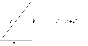
Remember Pythagoras? We know his famous result:
A Pythagorean triple is any group of three
integers like 3,4,5 where the squares of the
first two add up to the square of the third:
32 + 42 = 52.
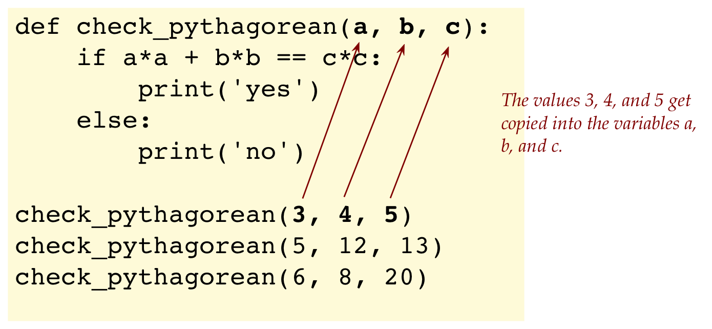
We'll now write code to check whether a trio of numbers
is indeed a Pythagorean triple:
This time, we've defined a method that takes three parameters:
def check_pythagorean(a, b, c):
    # Write your function code here
Notice the commas separating the three variables.
Consider the first invocation:
The invocation also uses commas to separate arguments.
2.7 Exercise:
In
my_func_example4.py,
fill in the code in the function below so that the output
of the program is:
5
3
2
0
The partially written program is:
def print_profit_total(a,b):
    # Write your function code here

print_profit_total(2, 3)
print_profit_total(-2, 3)
print_profit_total(2, -3)
print_profit_total(-2, -3)
The idea is to compute the sum but only of the positive parameters;
if neither value is positive, print 0.
2.8 Video:
2.3 Return values
So far, we've written methods that take values,
do things and print.
We get a whole new level of programming power, when
methods can compute something and return something
to the invoking code.
Here's an example:
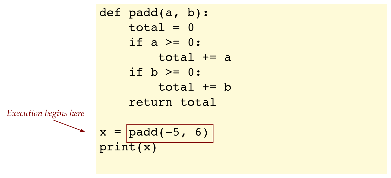
def padd(a, b):
    total = 0
    if a >= 0:
        total += a
    if b >= 0:
        total += b
    return total

x = padd(-5, 6)
print(x)
2.9 Exercise:
Type up the above in
my_func_example5.py.
Then try sending 5,-6 instead of -5,6. Then try 5,6.
In your module pdf, trace through the execution in each case.
What does the
padd()
function achieve?
Let's explain:
First, execution begins after the function definition is
"absorbed" by Python:
Remember, in an assignment statement, the right side
is executed first:
x = padd(-5, 6)
The result of invoking this function somehow results in
x
getting a value stored inside it.
(We'll see how, shortly.)
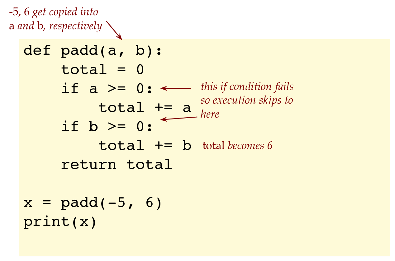
Next, execution goes into the function:
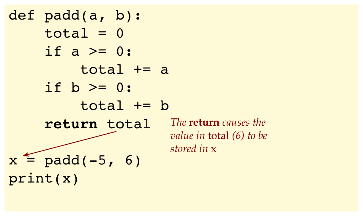
When the return statement executes, the value returned
(the value of
total)
gets copied into
x
One way to think about it:
When we see
x = padd(-5, 6)
then think of execution going to the function
padd
After it executes, it returns the value in one of its
variables: in this case 6
That, behind the scenes, replaces the function invocation:
x = 6
And thus, the value 6 gets copied into
x.
2.10 Exercise:
In
my_func_example6.py,
complete the code in
sum_up_to()
so that it computes and then returns the sum of numbers from 1 to n
(inclusive of 1 and n).
def sum_up_to(n):
    # write your code here

result = sum_up_to(5)
print(result)            # should print 15
result = sum_up_to(10)
print(result)            # should print 55
2.11 Video:
Let's return to our earlier example and use the
padd()
function in different ways:
def padd(a, b):
    print('Received values: ', a, b)
    total = 0
    if a >= 0:
        total += a
    if b >= 0:
        total += b
    return total

print(padd(-5, 6))
x = padd(padd(-5,6), 7)
print(x)
print(padd(padd(-5,6), padd(5,-6)))
2.12 Exercise:
Type up the above in
my_func_example7.py
and report what it prints in your module pdf.
Let's examine each of the last three statements:
The first one:
print(padd(-5, 6))
In this case:
The invocation to
padd()
occurs first:
print(padd(-5, 6))
That function executes and returns 6.
So, we can think of the result of that as:
print( 6 )
Which sends 6 to the
print()
function.
Which prints 6.
Next consider
x = padd(padd(-5,6), 7)
In this case:
The innermost
padd()
is first invoked:
x = padd( padd(-5,6), 7 )
That takes execution into
padd()
with parameter values
padd(-5, 6).
The function returns 6, and so, we could think of the result
as
x = padd( 6, 7 )
This now results in another invocation to
padd()
with parameter values
padd(6, 7).
The function now executes again and returns 13.
The result is
x = 13
Finally, consider the third example:
print(padd(padd(-5,6), padd(5,-6)))
In this case:
There are two innermost invocations:
print(padd( padd(-5,6), padd(5,-6) ))
The left one is called first:
print(padd( padd(-5,6), padd(5,-6) ))
Resulting in a return value of 6:
print(padd( 6, padd(5,-6) ))
Then, the other one is invoked, sending 5,-6 to the function:
print(padd( 6, padd(5,-6) ))
Which will cause 5 to be returned:
print(padd( 6, 5 ))
Now, these results (6 and 5) are sent once again to the
third invocation:
print( padd( 6, 5 ) )
This returns 11.
print( 11 )
And so 11 gets sent to print, which prints it.
Whew!
2.4 Multiple returns in a function
Take a moment to go back up and quickly glance through the Pythagorean example.
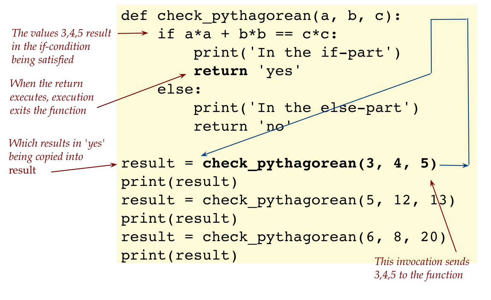
Now consider this rewrite:
def check_pythagorean(a, b, c):
    if a*a + b*b == c*c:
        print('In the if-part')
        return 'yes'
    else:
        print('In the else-part')
        return 'no'

result = check_pythagorean(3, 4, 5)
print(result)
result = check_pythagorean(5, 12, 13)
print(result)
result = check_pythagorean(6, 8, 20)
print(result)
2.13 Exercise:
Type up the above in
my_func_example8.py
and report what it prints in your module pdf.
Note:
Important: When a function executes a return
statement, execution exits the function right then and there,
even if there's more code below.
Thus for example, in the first time
check_pythagorean()
is invoked:
2.14 Exercise:
In your module pdf, draw such a diagram for
the other two function invocations.
2.15 Exercise:
In
my_func_example9.py,
complete the code below so that the function, when given
three numbers, identifies the two larger ones and returns their sum.
def add_bigger_pair(a, b, c):
    # Write your code here:

print(add_bigger_pair(2,3,4))  # Should print 7
print(add_bigger_pair(2,3,1))  # Should print 5
print(add_bigger_pair(2,1,4))  # Should print 6
2.16 Video:
2.5 Parameter and argument names
Consider this example:
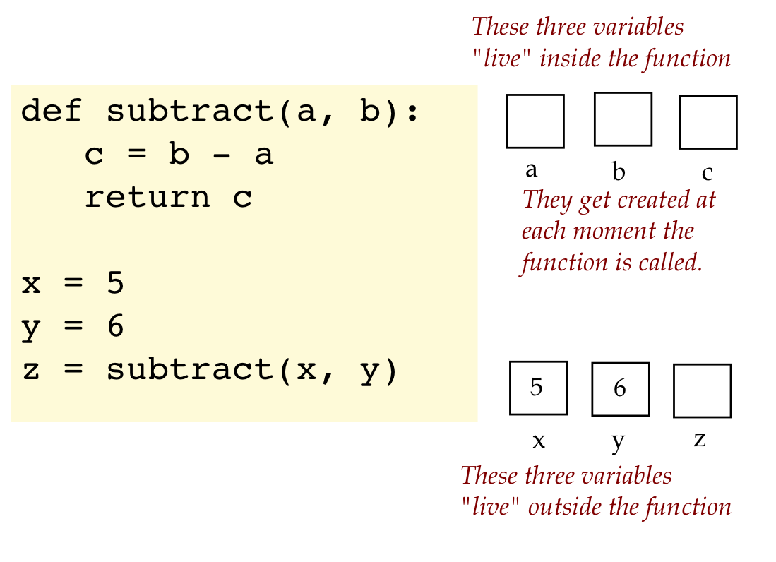
def subtract(a, b):
   c = b - a
   return c

x = 5
y = 6
z = subtract(x, y)
Note:
We refer to
a
and
b
as parameters in the definition of the function:
def subtract(a, b):
When function is invoked,
subtract(x, y):
we sometimes use the term
function arguments for
x
and
y.
The names given to parameters have no relation to
the names used for arguments:
In the above case:
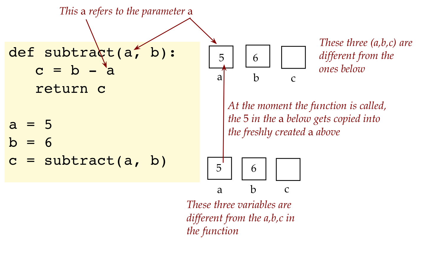
Consider this variation:
def subtract(a, b):
   c = b - a
   return c

a = 5
b = 6
c = subtract(a, b)
The a,b,c that are the parameter variables are
different from the a,b,c variables below:
Important: If you aren't sure, it's safest to use
different names.
2.6 What can you do with parameter variables?
Generally, the purpose of parameter variables is this:
Consider this example:
def silly_func(a, b):
    c = 2*a - b
    print(c)

silly_func(3, 4)
x = 6
silly_func(x, 8)
From the point of view of the function,
silly_func
thinks "Someone is going to put values into my variables a and b,
and then I'll do stuff like calculate and print".
From the point of view of code that is using the
function, as in
silly_func(3, 4)
This is saying "we'll set the function's a parameter to 3, and b
parameter to 4, and then let the function do its thing".
Now, functions can use its parameter variables just like
any other variable and change its value, as in:
def crazy_func(p, q):
    print(p)
    p = p + 3*q       # We're changing p here
    print(p)
    r = p + q
    print(r)

x = 6
y = 7
crazy_func(x, y)
Because the value in x gets copied into the variable p, the value
in x does not get changed even though the function changes the
value in p.
2.17 Exercise:
Just by reading, can you tell what the above program prints?
Then, implement in
my_func_example10.py
and confirm.
2.7 Functions and lists
Can a function receive a list as parameter? Can it return one? Is this
useful? Yes, yes, yes.
Let's start with a list as parameter:
def compute_total(B):
    total = 0
    for k in B:
        total += k
    return total

A = [1, 3, 5, 7]
t = compute_total(A)
print(t)
2.18 Exercise:
In your module pdf, trace the execution of the above program,
including loop iterations.
Type up the above in
my_func_example11.py,
including a
print(k)
in the loop to confirm your trace.
2.19 Exercise:
In
my_even_numbers.py,
complete the code in the function below so that
the even numbers in a list are printed out:
def print_even(A):
    # Insert your code here

A = [1, 3, 5, 6, 7, 8]
print_even(A)
Write the function so that the output is:
Found even:  6
Found even:  8
Recall how to use the remainder operator from the previous
module (conditionals and loops).
2.20 Audio:
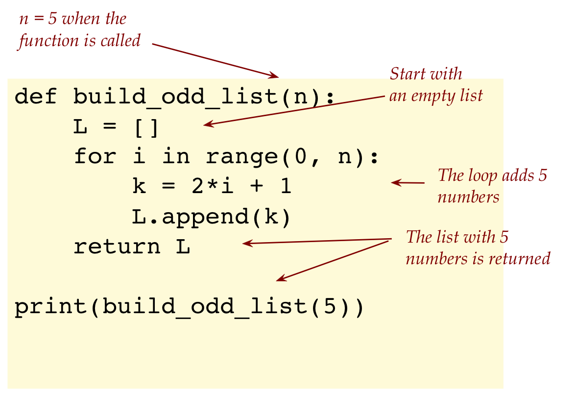
Next, let's look at an example where a list is returned:
def build_odd_list(n):
    L = []
    for i in range(0, n):
        k = 2*i + 1
        L.append(k)
    return L

print(build_odd_list(5))
2.21 Exercise:
Trace through the above in your module pdf, then type up in
my_odd_list.py
to confirm. Include a
print(k)
in the loop after the append.
Note:
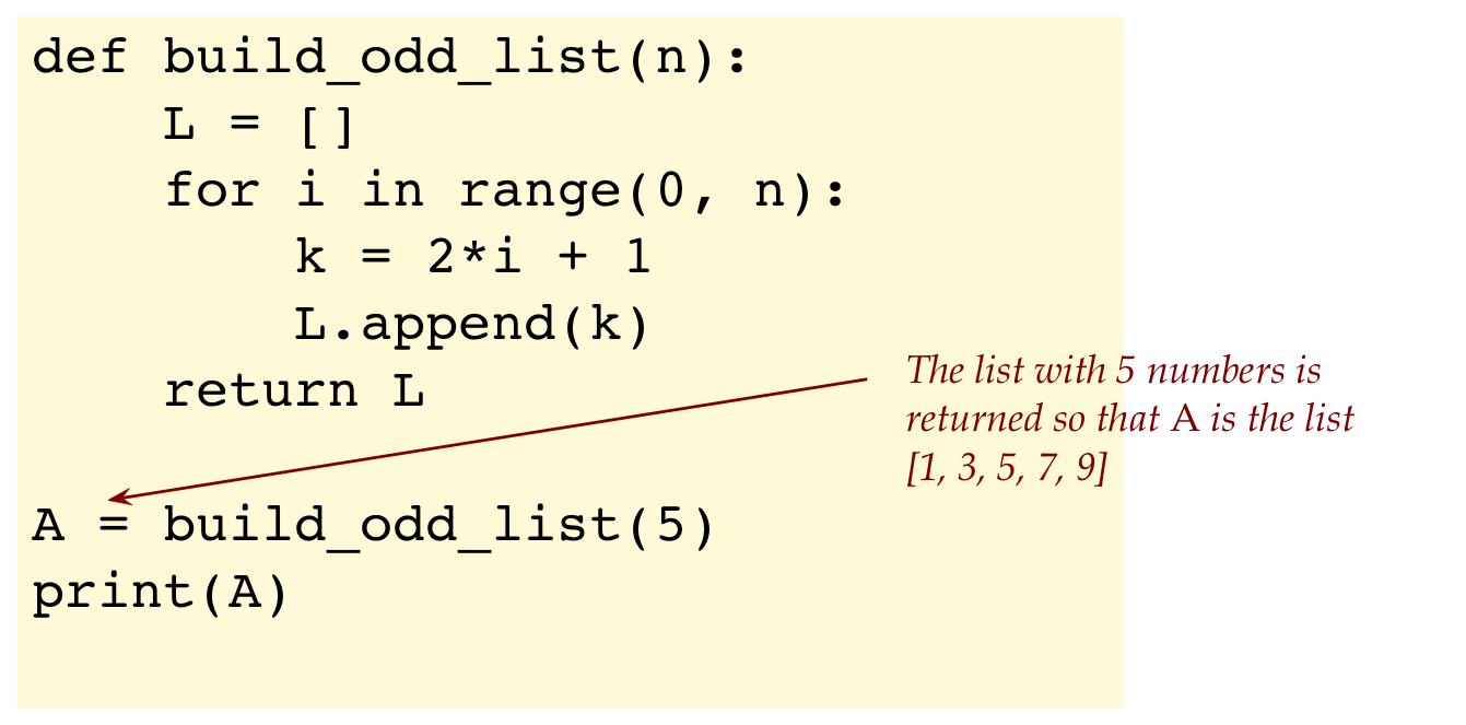
Execution begins with
print(build_odd_list(5))
This results in:
Once the return occurs, we could think of this as:
print( [1, 3, 5, 7, 9] )
This gets sent to print, which prints.
One could make this more explicit:
Next, let's look at a list example with multiple returns:
def find_first_negative(A):
    for k in A:
        if k < 0:
            # First try print(k) here
            return k
            # Then try print(k) here
    return 0

B = [1, 2, -3, 4, -5, 6]
C = [1, 2, 3, 4]

print(find_first_negative(B))
print(find_first_negative(C))
2.22 Exercise:
Before typing this up in
my_first_negative.py
to confirm,
try to trace through the program in your module pdf.
That is, use the tracing approach we've used before:
write out the values of variables and how they change from one
iteration to the next.
Then, replace the first comment so that you print(k) inside the loop.
Explain what you see as a result in your module pdf.
Then, move the print statement (still inside the loop) to
after the
return k
statement. What do you observe? Explain in your module pdf.
2.23 Exercise:
In
my_last_negative.py,
modify the above program to find the last negative number (if one
exists) in a list. So, after completing the code below
def find_last_negative(A):
    # Insert your code here

B = [1, 2, -3, 4, -5, 6]
C = [1, 2, 3, 4]
it should print
-5
0
2.24 Audio:
2.8 returns that don't return anything
Consider this program:
def print_first_negative(A):
    for k in A:
        if k < 0:
            print('Found: ',k)
            return
    print('No negatives found')

B = [1, 2, -3, 4, -5, 6]
print_first_negative(B)
C = [1, 2, 3, 4]
print_first_negative(C)
2.25 Exercise:
Type up the above in
my_first_negative2.py,
execute and observe the output. Then, trace through the
execution in your module pdf.
Let's point out:
Whenever a
return
statement is executed in a function, execution exits
the function right away.
When a
return
statement does not return a variable's value,
execution leaves the function but does not give a value
back to the invoking code.
Thus the
return
here:
def print_first_negative(A):
    for k in A:
        if k < 0:
            print('Found: ',k)
            return
    print('No negatives found')
does not return a value but merely causes execution to leave the
function and to back to just after where the function was invoked.
Although it's not needed, one could return at the
end of a non-value-returning function:
def print_first_negative(A):
    for k in A:
        if k < 0:
            print('Found: ',k)
            return
    print('No negatives found')
    return
Why do we have multiple return's in a function? Why not
always wait until execution reaches the end of a function?
It is very useful to be able to return from anywhere
in a function's code.
The reason is: as soon as the function's "job" is done
(example: finding the first negative), we want to leave the
function.
2.9 A fundamental difference between list and basic parameters
Consider this program:
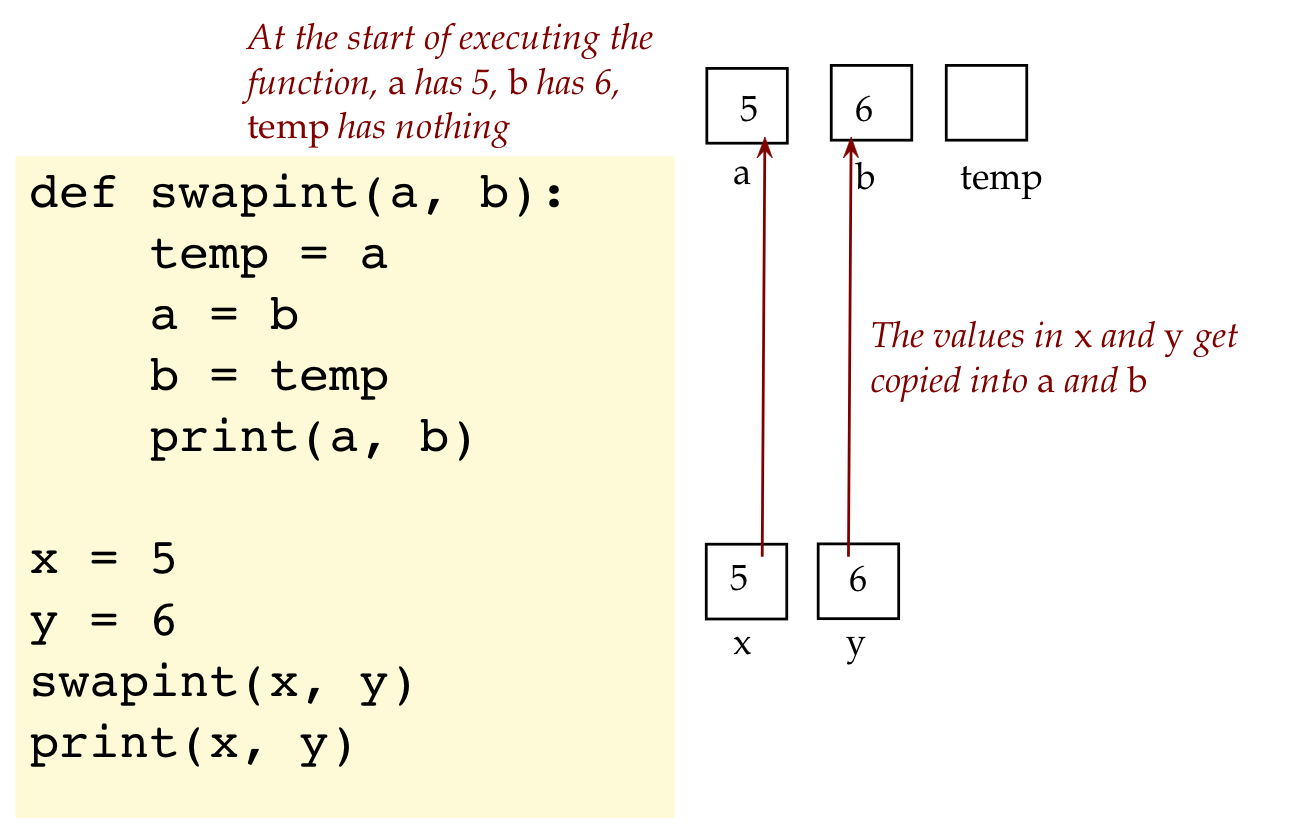
def swapint(a, b):
    temp = a
    a = b
    b = temp
    print(a, b)

x = 5
y = 6
swapint(x, y)
print(x, y)     # Will this print 5 and 6, or 6 and 5?
2.26 Exercise:
Before typing up the above in
my_swap_int.py,
can you guess what the output will be?
Let's explain:
Execution of the program begins with the line
x = 5
When the function is called soon after:
swapint(x, y)
then execution enters the function with the values in x and y
copied into a and b:
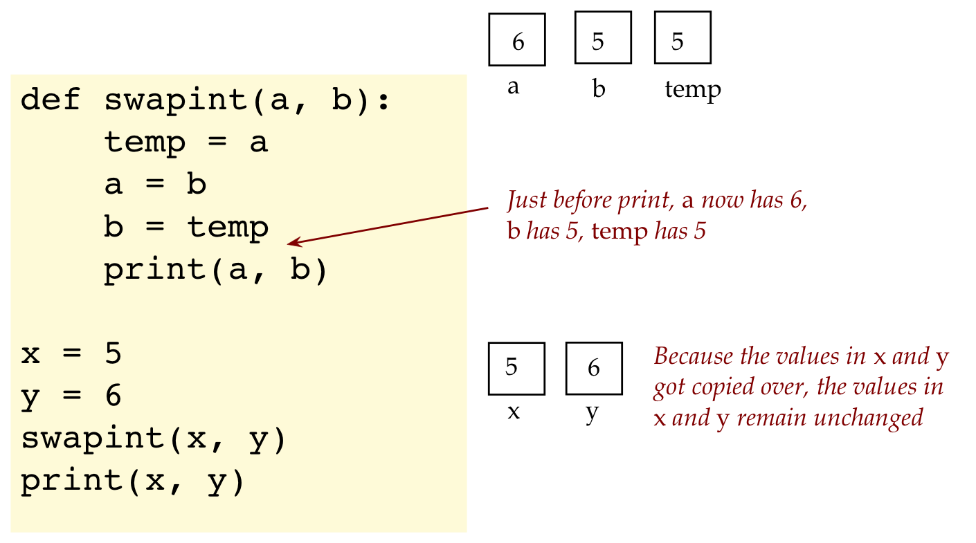
Then, by the time we reach the print statement:
Thus, the values in a and b do indeed get swapped.
But this does not affect x and y because they are
actually different variables.
2.27 Exercise:
In your module pdf, draw the three boxes for a, b, and temp,
at each step in the function's execution.
2.28 Exercise:
Before typing up the above in
my_swap_list.py,
can you guess what the output will be? Is it strange?
Let's see what's going on:
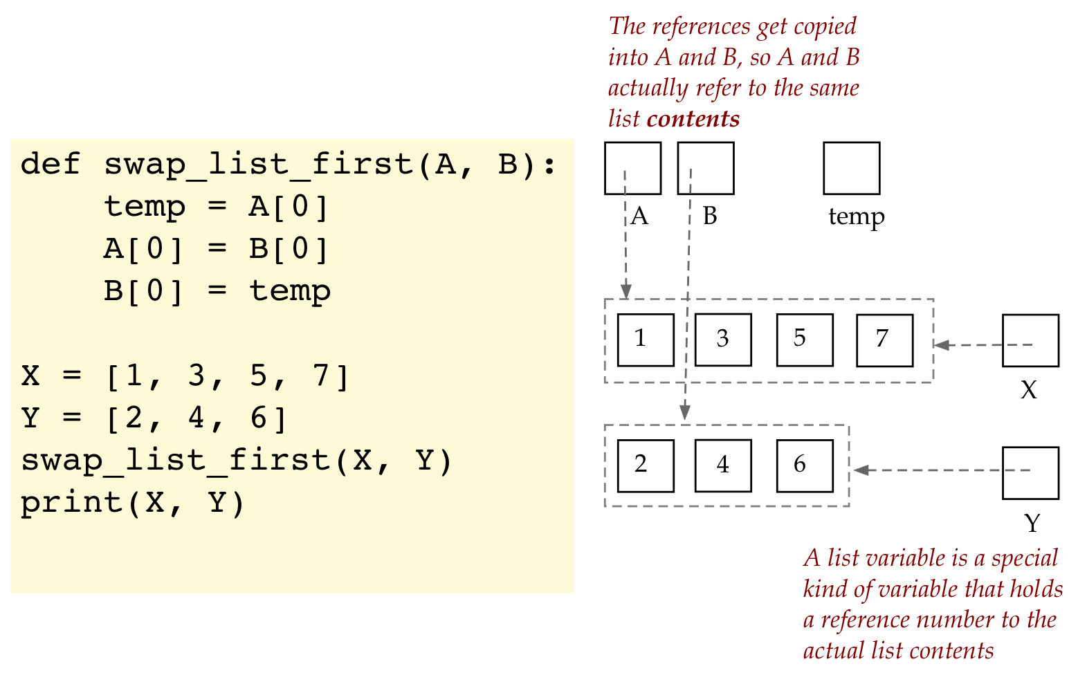
List variables are fundamentally different from numeric variables.
Think of a list variable has having a reference ID to
the actual list contents:
This is like an "address" in memory.
If you have this "address" you can go to the list
and do things with it.
List variables actual store these addresses (which,
interestingly, turn out to be numbers).
We will draw a conceptual diagram to highlight
this point:
Thus, when the function starts execution, the
"references" in X and Y are copied into A and B.
This means A and B refer to the same list contents.
So, A[0] is the same as X[0], for example.
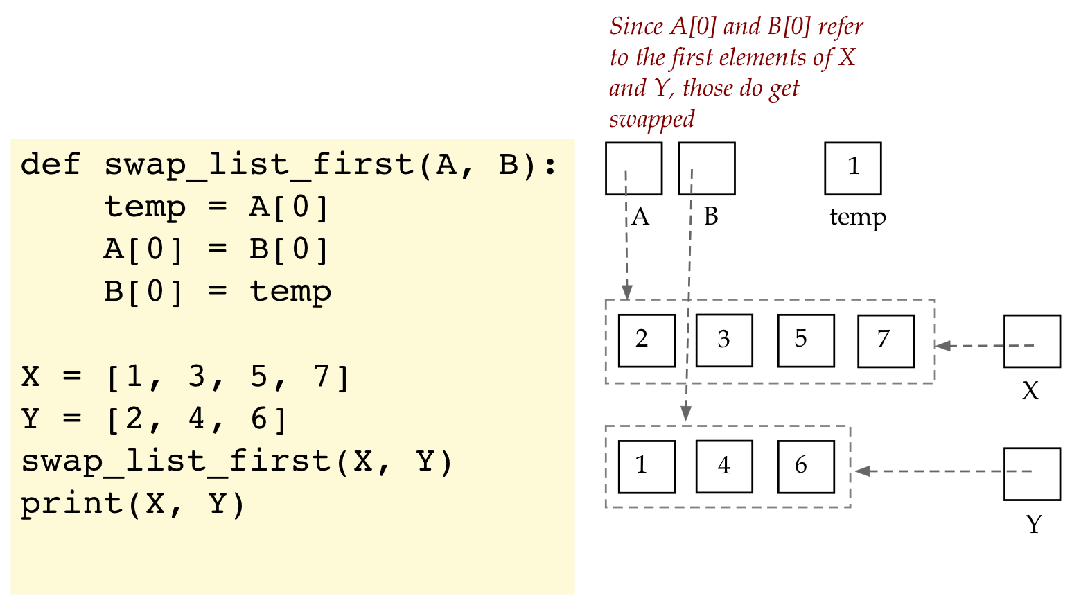
Next, after executing the three lines inside the function
but before returning:
Notice that temp is a regular integer.
2.29 Exercise:
In your module pdf, draw the above diagram after each line
in the function, showing how the list contents and temp
change with each line of execution.
2.30 Audio:
The key takeaways:
When you send number variables to a function, they get copied,
and so the function can't "do" anything to the variables you
present as arguments.
But if you send a list, a function can change the contents.
This means you need to be careful about intent
when writing functions that involve larger entities like lists.
(There are other such "grouped data" entities, called objects.)
If the intent is to change contents, that's fine, we should know
that.
2.31 Exercise:
Consider the following program:
def change_int(a):
    a = a + 1

def change_list(A):
    A[0] = A[0] + 1

x = 5
change_int(x)
print(x)

B = [1, 2, 3]
change_list(B)
print(B)
In your module pdf, trace through the above program, showing
boxes for the different variables changing as each line executes.
Show these diagrams at the start of each function's execution and
just before each function returns.
2.32 Audio:
2.10 Calling functions from functions
The code inside functions can be like regular
code that's outside functions.
In particular, code inside functions can call (invoke) other
functions.
For example:
def increment(a):
    b = a + 1
    return b

def increment_twice(c):
    d = increment(c)
    e = increment(d)
    return e

x = 5
y = increment_twice(x)
print(y)
Note:
The program starts execution at the line
x = 5
Then, when
increment_twice(x)
is called, we enter the function
increment_twice()
with the variable
c
set to 5 (copied from x).
The next line in there
d = increment(c)
results in a call to
increment()
with the value 5 copied into parameter
a.
Then, the code in
increment()
executes, resulting in 6 being returned.
The returned value 6 is stored in
d.
Then
increment()
is called again with the value in
d.
(now 6) copied into
a.
The code in
increment()
executes resulting in 7 returned.
Execution continues in the
increment_twice()
function and the value 7 is stored in
e.
Finally
increment_twice()
completes execution and returns the value in
e,
which is 7.
This value is stored in
y,
Execution continues from there to the print.
In addition, observe the following:
We can shorten the above code by writing:
def increment(a):
    return a + 1

def increment_twice(c):
    return increment(increment(c))

x = 5
y = increment_twice(x)
print(y)
Notice that one can return the result of
an expression:
return a + 1
In this case, the calculation is an arithmetic expression.
One can also have the result of a function call itself be
returned:
In the same vein, we can, instead of printing, execute a
return:
return increment(increment(c))
Note: you do NOT have to use such shortcuts. Some shortcuts
are an advanced topic and may in fact make your code harder to
read, and harder to fix mistakes in.
2.33 Exercise:
Consider the following program:
def decrement(a):
    return a - 1

def subtract(a, b):
    for i in range(0, a):
        b = decrement(b)
    return b

print(subtract(5, 9))
print(subtract(3, 13))
Type this up in
my_subtraction.py.
Then in your module pdf, trace the execution step by step.
Draw diagrams showing the changing contents of variables
a and b. (This exercise is a bit long, but worth doing because
it will help your understanding.)
2.34 Video:
2.11 More stats via programming
Armed with our new ability to work with functions and lists,
we will see how easy it is to compute basic statistics with data.
Before we get to that, here's a small exercise.
2.35 Exercise:
Consider the following program:
def find_smallest(A):
    smallest = A[0]
    for k in A:
        if k < smallest:
            smallest = k
    return smallest

data = [-2.3, -1.22, 1.6, -10.5, 1.4, 2.5, -3.32, 11.03, 2, 2, -1.4]
print(find_smallest(data))
Type this up in
my_find_smallest.py.
Then trace through the execution in your module pdf. It's critical
to understand how the variable
smallest
is changing through the loop, and why the function
find_smallest()
does in fact identify the smallest value in a list.
(Remember: the more negative a number, the smaller. Thus, -10 is
less than or "smaller" than -4.)
With that, consider this partially complete program:
def find_smallest(A):
    smallest = A[0]
    for k in A:
        if k < smallest:
            smallest = k
    return smallest

def find_largest(A):
    # Insert your code here:

def find_span(A):
    smallest = find_smallest(A)
    largest = find_largest(A)
    span = largest - smallest
    return span

data = [-2.3, -1.22, 1.6, -10.5, 1.4, 2.5, -3.32, 11.03, 2, 2, -1.4]
print('span: ', find_span(data))
2.36 Exercise:
In
my_stats.py
complete the above so that the span of the data
is computed and printed. This is the difference between
the largest and smallest values.
Then, use a table (as you have before) to trace through
the execution in your module pdf.
2.37 Video:
Next, let's write some (partially complete) code for standard statistics:
import math

def compute_mean(A):
    # Insert your code here:

def compute_std(A):
    mean = compute_mean(A)
    total = 0
    for k in A:
        total += (k-mean)**2
    std = math.sqrt( total / len(A) )
    return std

data = [-2.3, -1.22, 1.6, -10.5, 1.4, 2.5, -3.32, 11.03, 2, 2, -1.4]
print('mean =', compute_mean(data))
print('standard deviation =', compute_std(data))
Note:
The mean of a list of numbers is the total (add the
numbers up) divided by "how many numbers there are" in the list.
The standard deviation is more involved:
Consider data like:
10, 20, 30, 40, 50
This is centered around 30 (mean in this case).
Here, a different set of data that's also centered around 30:
28, 29, 30, 31, 32
Clearly, the second set of data is very bunched up around 30
while the first is more spread out.
The standard deviation is a measure (a single
number) that rates the "spreadout-ness" of data.
The more spread out, the higher the standard deviation.
To calculate it, we take the difference of each data
from the mean, square it (to make it always positive),
then add all of these up.
This gives something called the variance,
which itself is a fine measure of spreadout-ness.
However, because we're adding up squared numbers, the
variance can become a big number.
To bring the measure closer to the "level" of the actual
data, we take the square root of the variance: this is
the standard deviation.
If you've never seen this before, it's worth computing
by hand with the data above, just so you understand how it looks
on paper. Then compare with the results from the program.
2.38 Exercise:
In
my_stats2.py
complete the code above. You should get as output, approximately
mean = 0.1627272727272727
standard deviation = 4.955716792313685
(Real numbers, what can you do?)
Next, let's tackle the more challenging problem of identifying
outliers:
We see that two data values seem to be far outside the range of
the other data.
Suppose we use the following approach to identifying outliers:
Compute the mean and standard deviation.
Identify those data that lie further than two standard deviations
away from the mean.
Call these outliers.
Note: the traditional definition uses three standard
deviations, but we'll stick with two because it makes our example
easy to work with.
Let's write a function to do this:
def find_outliers(A):
    mean = compute_mean(A)
    std = compute_std(A)
    for k in A:
        if k < (mean - 2*std):
            print('Found outlier: ', k)
        elif k > (mean + 2*std):
            print('Found outlier: ', k)
2.39 Exercise:
In
my_stats3.py,
add the above to your code from the earlier exercise so that
the output is:
mean = 0.1627272727272727
standard deviation = 4.955716792313685
Found outlier:  -10.5
Found outlier:  11.03
2.12 A function that calls itself
This is a somewhat advanced topic (not on any exam or
assignment!).
We will only present a simple example only so that you see
what it's like.
Consider this example:
def factorial(n):
    # print(n)
    if n == 1:
        return 1
    else:
        m = factorial(n-1)
        return n * m

print(factorial(5))
print(factorial(10))
2.40 Exercise:
Type up the above in
my_factorial.py.
Then, in your module pdf trace through what happens when
factorial(5)
is called. Remove the # symbol so that the print prints.
Let's point out:
Yes, it's allowed for a function to call itself.
Such a function is called a recursive function,
and the resulting behavior is called recursion.
The above example computes numbers like
1 × 2 × 3 × 4 × 5 × = 120
(This ascending multiplication is called factorial.)
For recursion to work, the successive calls to itself
have to end so that we don't get the infinity of barbershop mirrors.
In the above case, n eventually becomes 1. In this case,
there's no further call to itself.
Recursion is hard to understand, and will be featured
in later courses after you've got more programming under your belt.
Surprisingly, many problems are solvable elegantly and
efficiently using recursion.
It is possible to do recursion improperly, in which case
a program is set up to recurse forever. In this case, Python
will give up after too many recursions.
2.41 Video:
2.13 Incribed geometric figures as art
Of course we're going to try and use functions and
drawing.
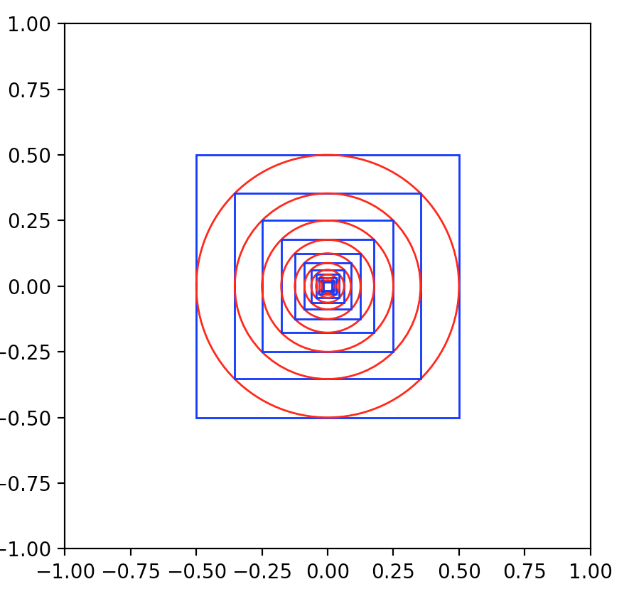
Consider this program:
import math
from drawtool import DrawTool

dt = DrawTool()
dt.set_XY_range(-1,1, -1,1)
dt.set_aspect('equal')

def draw_circle_in_square(side):
    radius = side/2
    dt.set_color('r')
    dt.draw_circle(0,0, radius)
    return radius

def draw_square_in_circle(radius):
    side = math.sqrt(2) * radius
    dt.set_color('b')
    dt.draw_rectangle(-side/2, -side/2, side, side)
    return side

side = 1
dt.draw_rectangle(-side/2, -side/2, side, side)

n = 5
for i in range(n):
    radius = draw_circle_in_square(side)
    side = draw_square_in_circle(radius)

dt.display()
Then, change n to n=10. Perhaps experiment
with colors. Try to read the functions and figure out, not so much
the calculation, as what they're doing.
At first, this looks like a simple exercise in geometric
art, or a depiction of the "evil eye" but there's more
to it:
Notice the construction:
We start with a square.
Then we inscribe the biggest possible circle
that'll fit inside that square.
Now we find the biggest possible square that'll fit inside
the recently drawn circle.
Then the square inscribed in that circle, and so on.
Instead of just using circles and squares, one can
use a square first, then a pentagon, then a hexagon, and so on.
The result is something that Kepler worked on a long time ago.
See this article
The historical significance is this:
Ever since the Greeks, polygons and circles have held
special significance.
So, something like this had an almost religious significance.
Kepler then used a similar idea for solids to expound
(an entirely wrong) theory of planetary motion.
To his credit, he realized he was wrong when shown higher
quality data (from Tycho Brahe), and used the data to fit ellipses.
This was the beginning of the modern understanding of
planetary motion, later mathematically solved by Isaac Newton.
2.14 When things go wrong
In each of the exercises below, first try to identify the error
just by reading. Then type up the program to confirm, and
after that, fix the error.
2.43 Exercise:
def square_it(x):
    y = x * x

a = 5
b = square_it(a)
print(b)
Identify and fix the error in
my_error1.py.
2.44 Exercise:
def bigger(x,y)
    if x > y:
        return x
    else:
        return y

print(bigger(4,5))
Identify and fix the error in
my_error2.py.
2.45 Exercise:
def find_smallest(A):
    smallest = 1000
    for k in A:
        if k < smallest:
            smallest = k
    return smallest

B = [2, 1, 4, 3]
print(find_smallest(B))
Does the above program work? What is the reasoning behind
the line
smallest = 1000?
What would go wrong if you removed it altogether?
Can you create a list (change the
data in B) which will cause the function to fail to find the smallest
number.
Fix the issue in
my_error3.py.