Understand how a list is different from a variable
Explore the syntax around using lists in programs
Use lists in programs to solve problems
Practice mental execution (tracing) and debugging related to lists
0.0 Audio:
0.0 An example of a list
Consider this program:
# List example:
A = [1, 4, 9, 16, 25]

for i in range(5):
    print(A[i])

# In contrast, a plain variable:
k = 100
print(k)
0.1 Exercise:
In
my_list1.py,
type up the above and examine the output. Then, inside the
above for-loop, but before the first print statement,
add an additional line of code to also print the value
of i so that each value of i is printed on a line by itself.
Report your output in
module0.pdf
and submit this modified version of my_list1.py.
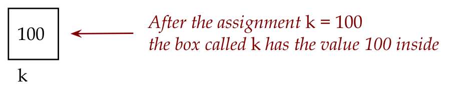
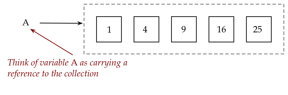
Remember how we think of a variable as a box that stores values?
This is indeed how we think of the variable
k
above.
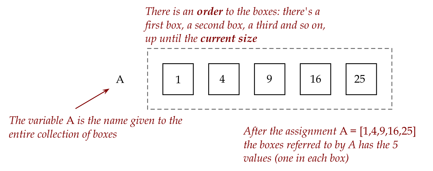
In contrast, a list variable is a single name given
to a collection of boxes:
The above collection has a current size, in this
case 5.
The values in a list are called elements of the list.
There is an implied order going from the first to the last element.
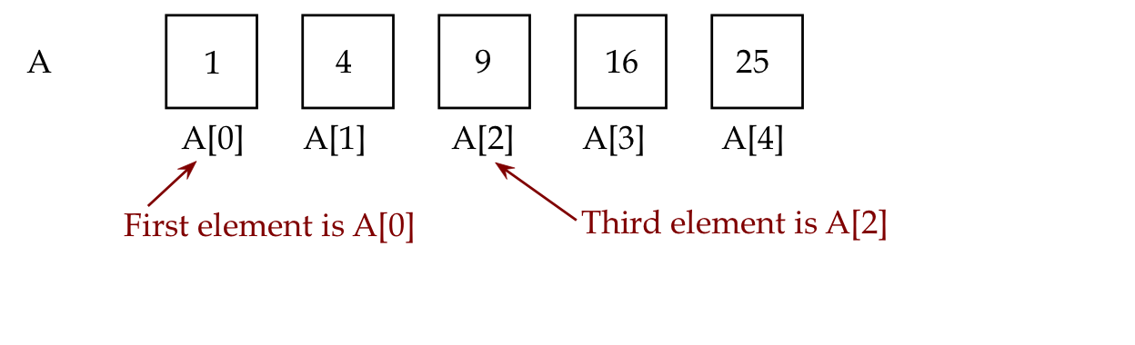
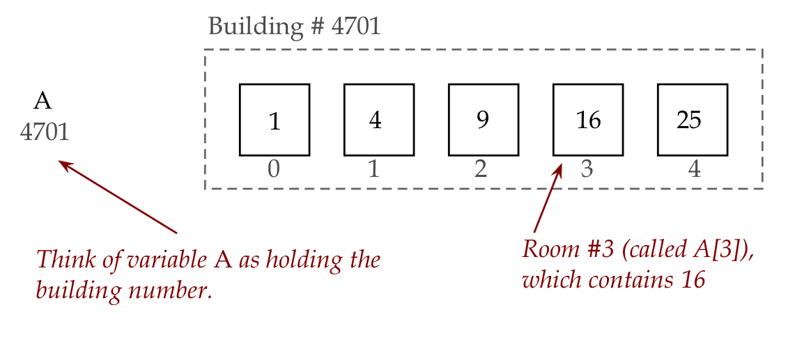
It turns out, we can access individual elements in the list
using indices:
Important:
List indices start at 0
And end at one less than the size.
Thus, in the above example, the size of the list is 5.
The indices (positions in the list) are: 0, 1, 2, 3, 4.
The last valid position (or index), which is 4 here,
is one less than the size, 5.
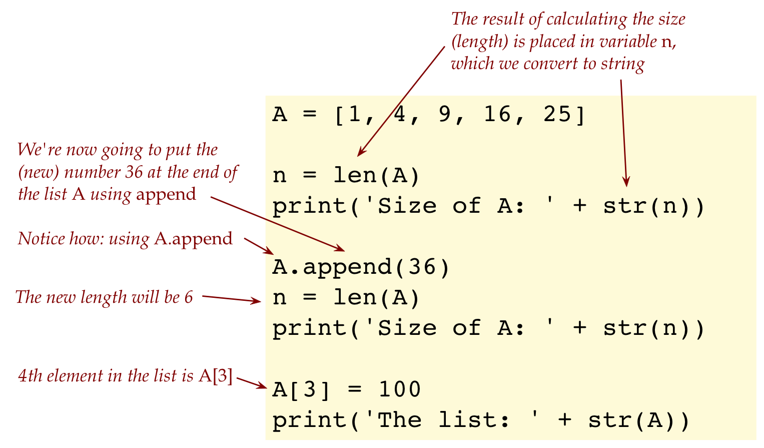
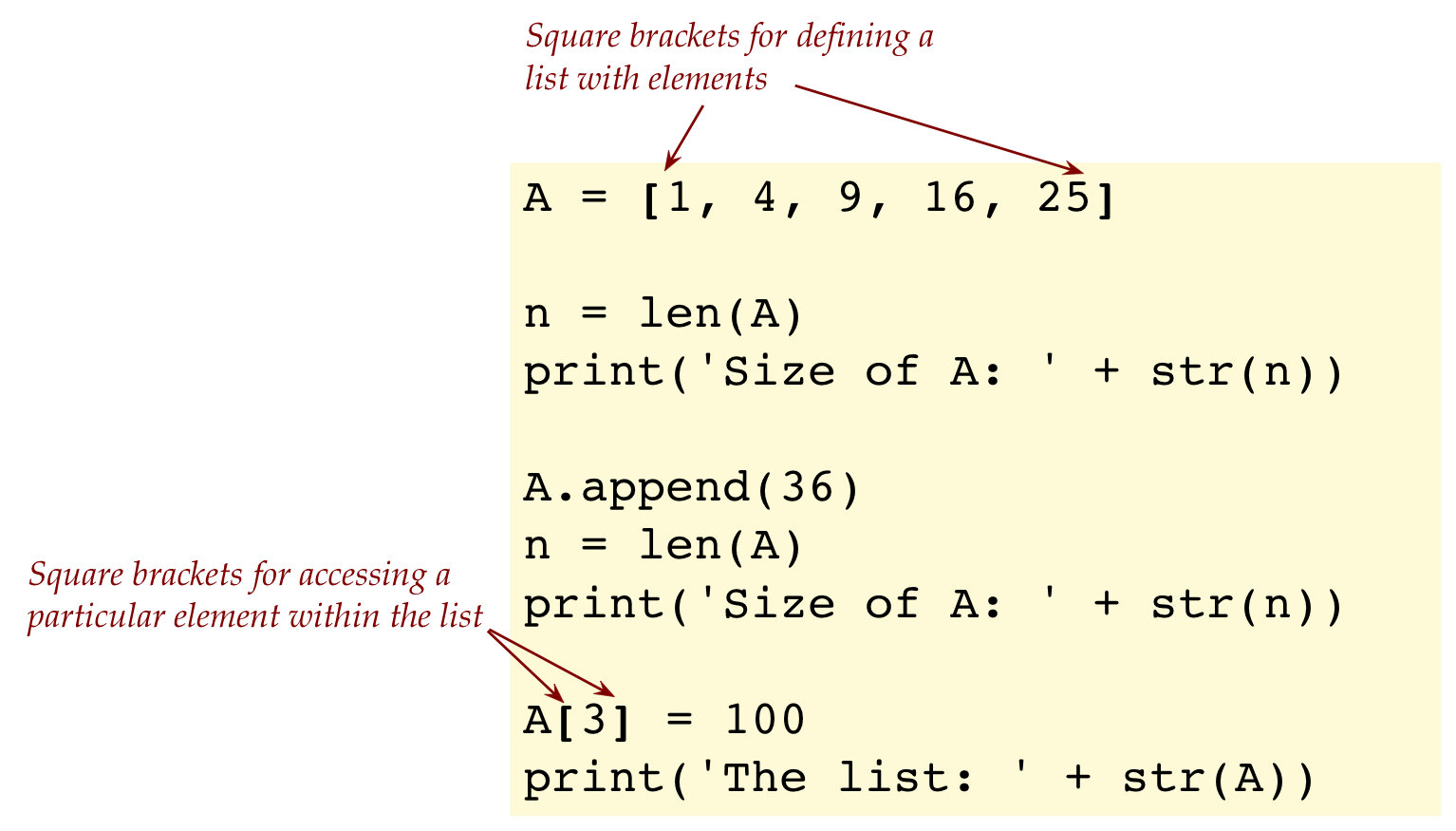
Consider this program:
A = [1, 4, 9, 16, 25]

# Use len to get the current size:
n = len(A)
print('Size of A: ' + str(n))

# Add an element to the list:
A.append(36)
n = len(A)
print('Size of A: ' + str(n))

# Change a particular element:
A[3] = 100
print('The list: ' + str(A))
0.2 Exercise:
Try out the above in
my_list2.py.
Let's point out:
Observe how we obtain the current size and add an element:
Next, observe square brackets being used for different purposes:
We could use a variable to access elements, as long as that
variable has an integer value that has a valid index, for example:
  k = 3
  A[k] = 100
Remember
len?
We had used
len
earlier for the length of strings, as in
s = 'hello'
print(len(s))    # Prints 5
Here,
len
works to give us the length of a list, as in:
A = [1, 4, 9, 16, 25]
print(len(A))
For example:
A = [1, 4, 9, 16, 25]

i = 3         # i's value 3 is valid for a size 5 list
print(A[i])

i = 7         # 7 is not valid
print(A[i])
In the above example, there is no element
A[7]
in a list that only has 5 elements.
0.3 Exercise:
Type up the above in
my_list3.py.
Describe the error in your module pdf.
0.4 Exercise:
In
my_list4.py,
make a list with the values 1,2,3,4,5,6,7,8,9,10. Then,
set up a for-loop so that only the odd numbers are printed as in:
1
3
5
7
9
0.5 Video:
0.1 More list examples
Just as we can add elements to list, so can we remove elements, as in:
A = [64, 9, 25, 81, 49]
print(A)

A.remove(9)
print(A)
0.6 Exercise:
Confirm the output by typing up the above in
my_list5.py.
Then, explore what would go wrong if you try and remove
something that's not in the list. For example, change
the line
A.remove(9)
to
A.remove(10).
Report what you see in your module pdf.
Submit your
my_list5.py
with the former (A.remove(9)).
Note:
The elements in a list do not need to be in sorted order, as
the above example shows. They can be in any order, but once
in that order, they stay in that order unless we make a change to
the elements in the list.
Although our examples so far have lists of integers like 64,
we will later build lists with real numbers and strings.
Consider this example:
# List constructed by typing the elements in:
A = [1, 4, 9, 16, 25]
print(A)

# List built using code to construct elements:
B = []                 # An empty list
for i in range(5):
    k = (i+1) * (i+1)
    B.append(k)
print(B)
0.7 Exercise:
Type up the above in
my_list6.py.
Then, in your module pdf, trace through the changing values
of i, k and the list B in each iteration of the for-loop.
Note:
It is possible to create an empty list and give it a variable
name as in:
B = [] # An empty list
We could then add elements by appending.
One can shorten the lines inside the loop:
B = []                 # An empty list
for i in range(5):
    B.append( (i+1) * (i+1) )
Here, we've fed the arithmetic expression
(i+1) * (i+1)
directly into
append,
without using a separate variable
k
to first calculate and then append.
0.8 Exercise:
In
my_odd_list.py
fill in the necessary code below to create a list with the first N
odd numbers:
N = 10
odd_numbers = []
# WRITE YOUR CODE HERE
print(odd_numbers)
In this case, the output should be:
[1, 3, 5, 7, 9, 11, 13, 15, 17, 19]
(These are the first 10 odd numbers).
0.9 Audio:
We do not need to traverse in exactly the order of elements in the
list:
For example:
A = [15, 25, 35, 45, 55, 65, 75, 85, 95, 105]

for i in range(9, 0, -2):
    print(A[i])
Here, we're starting at the last element, traversing the
list from end to beginning in steps of 2.
0.10 Exercise:
Trace through the above code showing the values of i
and A[i] at each iteration. Confirm by typing your code
in
my_list7.py.
0.2 A strange thing with lists
Let's first look at copying between regular variables, as in:
x = 5

y = x     # Copy the value in x into y

x = 6     # Change the value in x

print(y)  # Does it affect what's in y?
0.11 Exercise:
Consider the example above. In your module pdf, draw two boxes, one for x and one for y. Show the contents of the two boxes and if they change, show how they change.
Next, consider this:
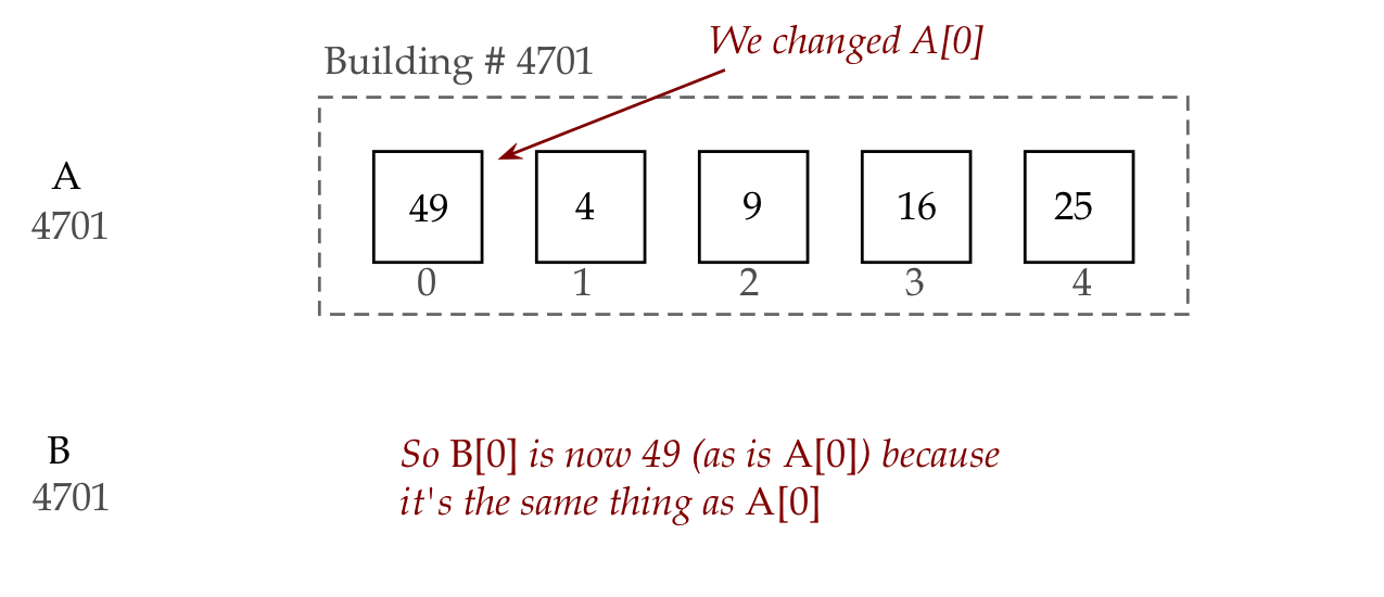
A = [1, 4, 9, 16, 25]

B = A

A[0] = 49    # Change some value in list A

print(B)     # Does it affect what's in list B?
0.12 Exercise:
Type up the above in
my_list_copy.py
to find out whether any values have changed in list B.
Let's explain:
Clearly something strange is going on with lists.
One way to think of it is to go back to our picture
of a list:
We'll now sketch out an analogy:
Think of the list as a building with rooms (the boxes):
Then, the list variable A is really something that
holds the building address (the building number).
The rooms in the building are numbered from 0, 1, etc.
The first room is A[0], the second is A[1] etc.
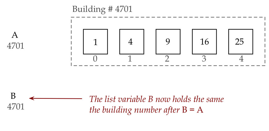
Now, consider an assignment like:
B = A
Then, in the building analogy, what we get is:
This is why, when we change the A list as in
A[0] = 49 # Change some value in list A
Then, we are achieving
Note: nowhere in our code is the building number (4701) explicitly
written. Building numbers (they are technically
called pointers) are handled by Python, and made invisible
to us because we don't need them.
(Yes, we can print the building number if we wish, but that's
an advanced topic.)
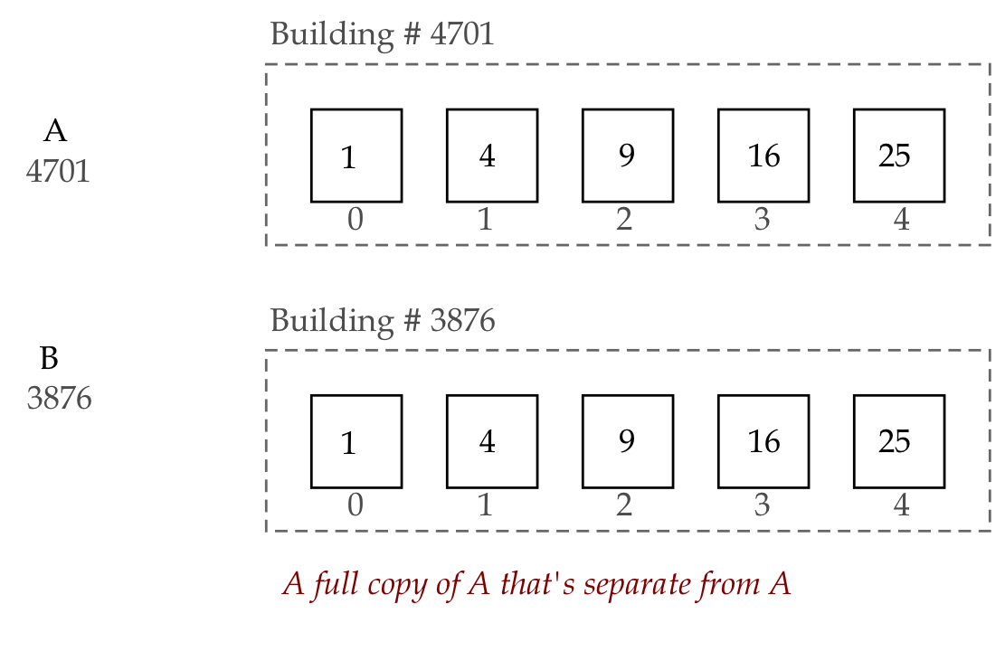
We obviously want to know: is it possible to create a
complete copy of A in B? As in:
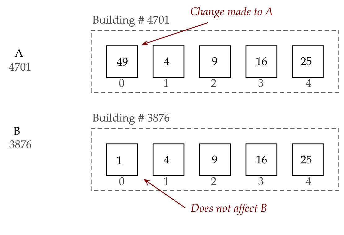
Because then, if we change A, it does not affect B:
This is what it looks like in code:
A = [1, 4, 9, 16, 25]

B = A.copy()

A[0] = 49    # Change some value in list A

print(B)     # Does it affect what's in list B?
0.13 Exercise:
Type up the above in
my_list_copy2.py
to find out if any values have changed in list B.
So, which (B = A
or B = A.copy()) do we use?
Generally, you should use
B.copy()
unless you intentionally want the same "building number".
In the former case, you have to be careful.
0.3 Different ways of iterating through a list
Consider this example:
A = [1, 3, 5, 7, 9]

total = 0
for i in range(5):
    total = total + A[i]

print(total)
0.14 Exercise:
Type up the above in
my_total_example1.py.
In your module pdf, trace through the values of i and total
through each iteration of the loop.
Now let's look at two different ways of writing the same loop
(we'll only show the loop part):
The first one:
for i in range(len(A)):
    total = total + A[i]
Notice:
Instead of figuring out the length of a list by looking at
the list, we can ask Python to compute the length and use that directly:
for i in range(len(A)):
    total = total + A[i]
This way, we don't need to track the length ourselves (if
elements get added or removed).
The second way is even better:
for k in A:
    total = total + k
Here:
Here the iteration is directly over the contents of the list.
The variable k is not an index but takes on the actual values
in the list.
With a list like
A = [1, 3, 5, 7, 9]

total = 0
for k in A:
    total = total + k
In the first iteration k is 1, in the second k is 3,
in the third k is 5, and so on.
So, naturally, these get added directly into the variable
total.
You can think of the first approach (using an index i and
A[i]) as index iteration.
The second (using the value directly), as content iteration.
Which one should one use?
Prefer to use content-iteration, whenever you can.
In some cases, however, you'll find
index iteration is useful, especially when
you need the position where something occurs in the list.
0.15 Exercise:
In
my_content_iteration.py,
use content-iteration to print the contents of the list A below:
A = [2020, 2016, 2012, 2008, 2004, 2000]

# Write your code here:
The output should be one number per line in the order that the numbers
appear in the list.
0.16 Audio:
0.4 Working with multiple lists
Suppose we have two lists of the same length like this:
A = [1, 4, 9, 16, 25]
B = [1, 3, 5, 7, 11]
Let's examine different ways of performing addition on the elements.
First, let's add up the total of all 10 numbers:
A = [1, 4, 9, 16, 25]
B = [1, 3, 5, 7, 11]

total = 0
for k in A:
    total = total + k

for k in B:
    total = total + k

print(total)
0.17 Exercise:
First, in your module pdf, trace the values of k and total in
each iteration of each loop.
Type the above in
my_twolist1.py
to confirm.
Note:
In the above case, we added all the numbers contained in both lists,
to get a single number.
Notice how natural it is to use content-iteration.
What if we want a third list whose elements are the
additions of corresponding elements from each list?
Let's write code to perform element-by-element addition:
A = [1, 4, 9, 16, 25]
B = [1, 3, 5, 7, 11]

C = []
for i in range(5):
    element_total = A[i] + B[i]
    C.append(element_total)

print(C)
0.18 Exercise:
First, in your module pdf, trace the values of i and
element_total in each iteration of the loop, and
also show how the list C changes across the iterations.
Type the above in
my_twolist2.py
to confirm. Print the list inside the loop, by adding
a print statement right after the append occurs.
(Submit your program with the added print statement.)
Explain why, in this case, index-iteration is a
better choice than content iteration.
0.19 Video:
0.5 Moving elements around in a list
Consider a list like:
A = [1, 4, 9, 16, 25]
Next, suppose we want to swap the elements in the 2nd and 4th
positions within the same list (not creating a new list).
That is, we want to write code so that:
A = [1, 4, 9, 16, 25]

# ... code to swap 2nd and 4th elements ...

print(A)

# Should print [1, 16, 9, 4, 25]
0.20 Exercise:
In your module pdf, trace through the execution above
showing the values in temp and the list after each line executes.
Then, do the same if the middle three lines were replaced by:
A[1] = A[3]
A[3] = A[1]
0.21 Exercise:
Use the "temp" variable idea to perform a left-rotate of a list in
my_left_rotate.py.
Thus, given
A = [1, 4, 9, 16, 25]
# ... your code here...

print(A)
# Should print [4, 9, 16, 25, 1]
Thus everything but the first element moves leftwards and the first
element gets to the last place. Use a for-loop to move most (but not
all) elements.
0.22 Audio:
0.6 Lists of strings, characters, or real numbers
We have thus far seen lists of integers.
One can make a list of other kinds of elements.
For example:
# A list of strings:
A = ['cats', 'and', 'dogs']
s = ''
for w in A:
    s += w
print(s)

# A way to extract the characters in a string into a list:
s = 'abcdef'
B = list(s)
print(B)

# Some real numbers:
C = [1.1, 2.22, 3.333, 4.4444]
total = 0
for x in C:
    total = total + x
print('Average =', total/4)
0.23 Exercise:
Type the above in
my_other_lists.py,
while noticing the subtle change in how the last print statement is written.
Insert spaces in the first loop so that the first thing printed is
cats and dogs.
0.7 A different version of print
Consider these two variations of using print:
x = 2
s = 'eat'
y = 3.141

print('I love ' + str(x) + ' ' + s + ' ' + str(y))

print('I love', x, s, y)
0.24 Exercise:
Type the above in
my_print_example.py,
Note:
The first version above uses string concatenation to
send one big string to print:
print( 'I love ' + str(x) + ' ' + s + ' ' + str(y) )
In the second version above, strings and variables
given to print are separated by commas.
Here, print treats the four things as separate entities:
print('I love', x, s, y)
In this case, print automatically inserts a space
between the different things (that are separated by commas).
In the second type, there is no need to convert numbers to strings.
0.8 Random selection of elements from a list
It is often useful to be able to pick random elements from
a list.
Let's use this feature first for a single roll of a die, and
then two dice:
Since a single die has 6 faces with the numbers 1 through 6,
we'll use a list of the numbers 1 through 6:
die = [1, 2, 3, 4, 5, 6]
Our goal is to choose one of these numbers randomly.
Python provides a way to randomly pick (without removing)
an element from a list:
die = [1, 2, 3, 4, 5, 6]
roll = random.choice(die)
Let's put this together into a program (remembering to
import the random package):
import random

die = [1, 2, 3, 4, 5, 6]
roll = random.choice(die)
print(roll)
0.25 Exercise:
Type the above in
my_die_roll.py.
Run the program several times to see that you are getting
random selections from the list.
Next, let's use this to make a (ridiculously) simple game:
Two players each roll a die N times. The numbers on the
rolls are averaged. The player with the higher average wins.
OK, not the most entertaining game, but one for which
we can easily write a program (from the point of view of one player):
import random

die = [1, 2, 3, 4, 5, 6]

num_trials = 10
total = 0
for i in range(num_trials):
    roll = random.choice(die)
    print(roll)
    total += roll

print('Average score:', total/num_trials)
0.26 Exercise:
Type the above in
my_die_roll2.py
to observe the result. Report in your module pdf the average when you use a
large number of trials (say, 1000).
0.27 Exercise:
In
my_die_roll3.py,
change the game to the following: in each trial,
each player rolls the die twice and adds the two numbers.
The final score is the average across all trials.
What is the average when you use a
large number of trials (say, 1000)?
In your module pdf, devise a more interesting 2-player game one
could play solely using dice. (You don't have to write
a program for this last part.)
0.28 Audio:
0.9 Some math via programming
Let's start with an example and then use that to delve
into a few concepts:
0.29 Exercise:
Type up the above in
my_plot_example.py
to see what you get.
You will also need to download
drawtool.py
into the same folder
Now let's ask some basic questions:
What, really, is a graph and what does it mean to plot on a graph?
What are x,y values and what do they have to with plotting?
What's a function and what's the connection between \(f(x)\)
and points on a graph?
And what does this have to do with programming?
We'll address these questions below.
Let's recall where we started:
In the beginning, there were integers (whole numbers) like 1,
2, 3, and 42.
Along with them came real needs like addition, subtraction,
multiplication and division.
(Ancient applications: navigation, telling time, accounting/trade).
The integers were not enough because you can perform
3 - 8 and get ... what? So came the negative integers like -5.
Then, because 5/2 is not an integer, more numbers were
needed, and hence the real numbers.
Next came algebra:
Instead of saying "I can take 12 times 4 and get 48, and
then divide by 6, to get twice your original number 4",
we can write: \(\frac{12x}{6} = 2x\)
It's much more compact and precise.
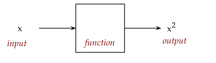
Next came functions:
Instead of saying "OK, take your number and multiply it by itself",
it's much more compact to say: \(f(x) = x^2\).
We can think of a function as taking some input (like \(x\)
and "doing something to it" to get an output:
All of this resulted in significant advances in mathematics.
Then came Descartes who took this to a whole new level with
coordinates.
The idea of coordinates:
Suppose you had a way of linking or associating pairs of
numbers:
For example, suppose 1 is associated with 5
2 is associated with 7
3 with 9
Suppose we wrote these as:
(1,5), (2,7), (3,9) and so on.
Next, draw two perpendicular lines (one horizontal, one
vertical) on a page:
And call them the x and y axes respectively.
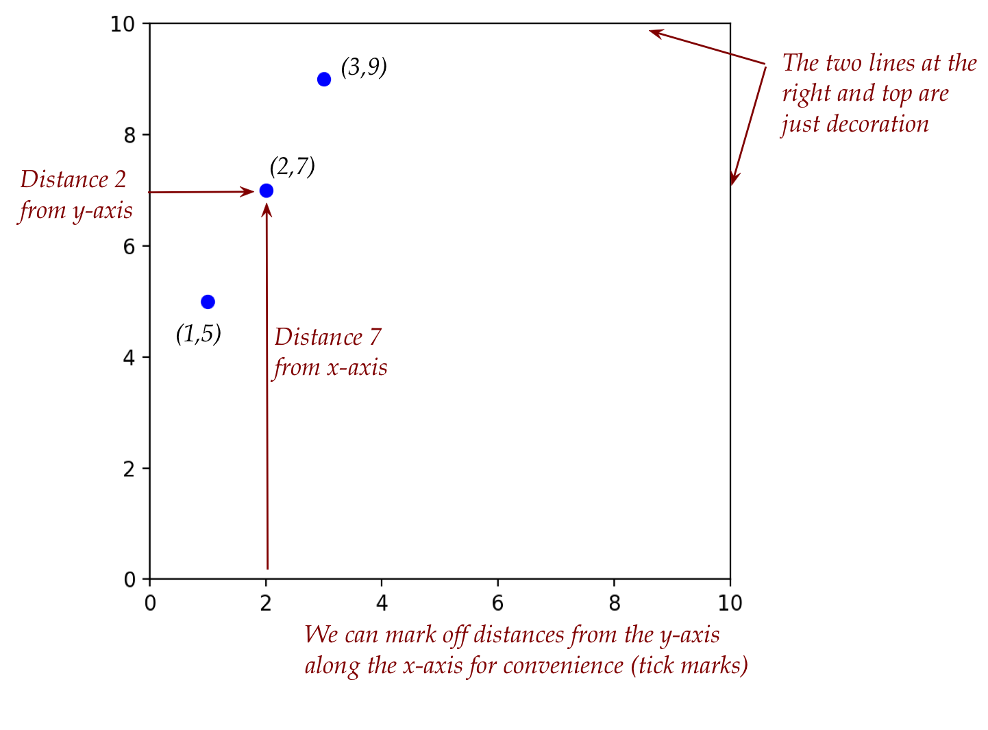
Now given associations (1,5), (2,7) and (3,9):
Treat the first number as the distance from the vertical axis.
Treat the second number as the distance from the horizontal axis.
This will put us in a unique spot.
Call that a point.
For example:
That's all there's to it. It's hard to believe that such a
simple idea became transformational.
The connection between functions and coordinates:
Suppose you have a function like: \(f(x) = 2x + 3\)
One way to make sense of a function is to compute
lots of examples like:
\(f({\bf 1}) = 2*{\bf 1} + 3 = 5\)
\(f({\bf 2}) = 2*{\bf 2} + 3 = 7\)
\(f({\bf 3}) = 2*{\bf 3} + 3 = 9\)
And even \(f({\bf 3.16}) = 2*{\bf 3.16} + 3 = 9.32\)
A pair of axes makes it possible to visualize
a function directly, initially by plotting some example
points:
Take some \(x\).
Calculate \(f(x)\)
Then treat \(x\) as the first coordinate (distance from y-axis).
Treat \(f(x)\) as the second coordinate (distance from
x-axis), and plot.
For example, when \(x=2\), then we saw that \(f(2) = 7\).
So, plot (2, 7).
In general, we want to plot \(x, f(x)\) for lots of
different possible \(x\) values.
Here, \(f(x)\) is what we use for the y-coordinate, which
is why we sometimes write \(y = f(x)\).
When we plot \(x, f(x)\) for different \(x\) values,
we typically pick those \(x\) values for our convenience.
For above, we showed how to calculate \(f(x) = 2x + 3\)
when \(x=1\),
when \(x=2\),
when \(x=3\),
and so on, perhaps up to
when \(x=10\),
(Here, the intended range is close to zero.)
But if we need to, we could just as easily calculate
\(f(x) = 2x + 3\)
when \(x=0.1\),
when \(x=0.2\),
when \(x=0.3\),
and so on up to when \(x=1.0\),
(Here, the intended range is close to zero, between 0 and 1.0)
Let's put these ideas to use:
Suppose we have two functions \(f\) and \(g\)
\(f(x) = 2x + 3\)
\(g(x) = x^2\)
Our goal: compare the two functions.
One advantage of programming is that we can write
code to perform the action of functions.
For example:
x = 0
for i in range(11):
    f = 2*x + 3
    print('x =', x, ' f(x) =', f)
    x = x + 1

x = 0
for i in range(11):
    g = x*x
    print('x =', x, ' g(x) =', g)
    x = x + 1
0.30 Exercise:
Type up the above in
my_function_example.py.
It is far more valuable to visualize, so let's set about plotting
both together:
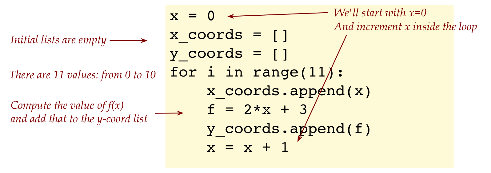
To plot, we'll need to construct the list of x and y coordinates:
from drawtool import DrawTool

dt = DrawTool()
dt.set_XY_range(1,10, 0,100)

x = 0
x_coords = []
y_coords = []
for i in range(11):
    x_coords.append(x)
    f = 2*x + 3
    y_coords.append(f)
    x = x + 1

dt.draw_curve_as_lines(x_coords, y_coords)

dt.set_color('r')

# WRITE CODE HERE for the second function

dt.draw_curve_as_lines(x_coords, y_coords)

dt.display()
Let's point out:
0.31 Exercise:
Type up the above in
my_function_plot.py
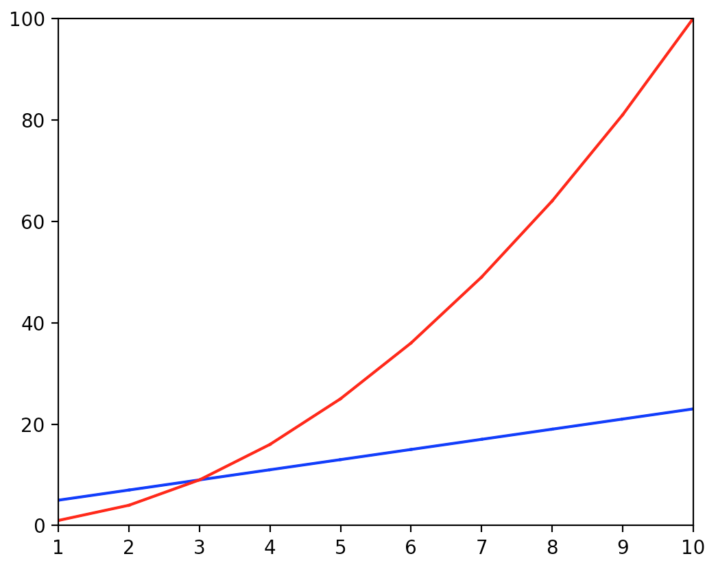
and add code for the second function \(g(x)=x^2\) to get
a plot like:
0.32 Video:
Scale and axes:
You may have noticed that the x-axis above had tick marks going
from 0 to 10, while the y-axis went from 0 to 100.
This is an example of a plot that's NOT drawn to scale.
Let's draw one to scale to see what it looks like by
changing one line, from
dt.set_XY_range(1,10, 0,100)
to
dt.set_XY_range(0,100, 0,100)
0.33 Exercise:
In
my_function_plot2.py
change your code from the earlier exercise to make the
scale the same along x and y axes.
When to use different scales along the axes:
Using the same scale, we see the dramatic difference between
linear growth (the function \(f(x)=2x+3\)) and
quadratic growth (the function \(g(x) = x^2\)).
But at the same time, some features like the point of
intersection of the two curves is hard to see.
We can use different scales when we want to emphasize
different aspects.
0.34 Exercise:
In
my_function_plot3.py,
add a third function \(h(x) = 2^x\).
Plot and take a screenshot once with the x and y range both as
[0, 1200], and once with the x-range as [0,12] and the y-range
as [0,1200].
This should show you how puny quadratic growth is compared
to exponential growth.
Submit your
my_function_plot3.py
with the former case when both ranges are the same.
0.10 Mathematical art
Since we're on the topic of functions, we cannot resist
developing an art project based on it.
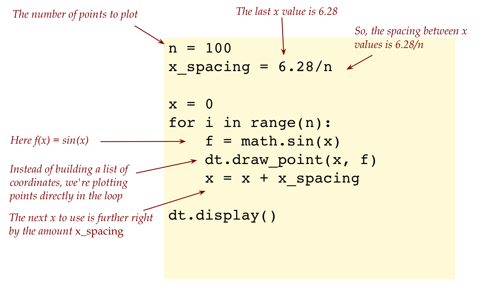
Let's first plot a function from high-school: the sine function
from drawtool import DrawTool
import math

dt = DrawTool()
dt.set_XY_range(0,6.28, -1,1)

n = 100
x_spacing = 6.28/n

x = 0
for i in range(n):
    f = math.sin(x)
    dt.draw_point(x, f)
    x = x + x_spacing

dt.display()
Let's point out:
First, some code features:
Next, observe that we plotted points directly inside the
loop instead of first building a list of coordinates.
Doing so is an alternative way of plotting ("plot as you go"),
and will let us change the point color.
So, for our art project:
We'll draw a background with randomly strewn yellow dots.
Then, along a sine-curve, we'll draw small ellipses of
different sizes.
0.35 Exercise:
Download functional_art.py
and run to see. Then in
my_functional_art.py,
improve on the above by including your own functions
and additional decoration by drawing.
0.11 When things go wrong
In each of the exercises below, first try to identify the error
just by reading. Then type up the program to confirm, and
after that, fix the error.
0.36 Exercise:
A = [1, 2, 3, 4, 5, 6, 7, 8, 9, 10]
for i in range(1, 10):
    print(A[i])
Identify and fix the error in
my_error1.py.
0.37 Exercise:
The following program intends to build the decreasing-order
list [10, 9, 8, 7, 6, 5, 4, 3, 2, 1].
A = []
n = 10
for i in range(n):
    n = n - 1
    A.append(n)

print(A)
Identify and fix the error in
my_error2.py.
0.38 Exercise:
The following program intends to add to N all
the elements of the list A.
N = 100
A = [1, 4, 9, 16, 25]

for k in A:
    N = N + A[k]

print(N)
Identify and ix the error in
my_error3.py.
0.12 Meta
This is the next installment in our series of
stepping back from it all and reflecting, with the hope
of helping you progress as a learner.
This time our topic is math and math anxiety.
Let's start by acknowledging a few things:
Students do in fact have bad experiences learning math.
For example, if you were unlucky to be ill during
the critical period in 4th grade when fractions are covered,
that could become a gap that precludes other concepts.
Or if algebra did not go well, everything that follows in math
can lead to cascading difficulties in learning.
Students learn math differently and their "window of
opportunity" may not be aligned with where their school is.
Thus, for many students, a certain age is not optimal
for academic intensity, or issues at home prevent full engagement.
There are hidden cultural dispositions that can get in the way.
The most pernicious by far is the notion that some people
just aren't cut out for it. Or you have to have the "math gene".
Much of K-12 math is, admittedly, a bit dull.
At the same time, there's good news:
Math (and programming) is like any other skill: everyone
can acquire it with sufficient practice, but not everyone can
reach the level of "world expert".
This is true of just about any mental skill: facility with
language, playing a musical instrument,
And, most importantly, anyone can acquire it at any age.
Can you tell someone it's too late to learn, say, French?
It all depends on shedding the "I'm not cut out for it" disposition
and committing to practice.
There is world of elegance and beauty in math after crossing
a threshold of skill level, just as with a musical instrument.
Let's say a bit more about practice:
You surely know a musical instrument cannot be learned merely
by watching videos or reading about it.
Proficiency requires regular and intense practice.
The best part of practice is that, even though progress
is not instantaneous, you can see results after a while.
Another advantage: the nature of practice is that
many people give up. So, if you don't, you are ahead of those that do.
Finally, the connection between programming and math:
It is true that most people who program do not use math at all.
Just ask a web developer.
But if you add a bit of math, you can do many interesting
things in programming, as anyone who deals with data will tell you.
Some aspects of computer science that have a strong mathematical
underpinning are just ... a lot of fun!