By the end of this module, for simple HelloWorld-like
programs, you will be able to:
Create variable declarations.
Assign values to variables by simple assignment, and print them out.
Distinguish between integers in strings versus actual integers.
Demonstrate ability to perform operations on integers
for a desired output.
Simplify expressions with constants to single value.
Evaluate expressions with variables in them.
Convert English descriptions of operations into expressions.
Mentally trace execution with expressions and calculations.
Mentally trace expressions and calculations inside for-loops.
Produce desired output using for-loops and calculations.
Identify new syntactic elements related to the above.
And, once we've worked with integers, we'll also do some
"number crunching".
4.0 Audio:
4.0 First, an analogy
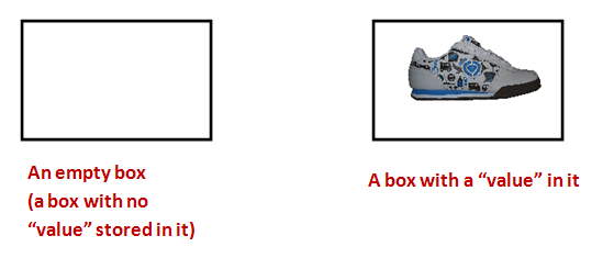
Suppose we have boxes. Consider the following rules about "boxes":
Each box can store only one item.
The possible things that can be stored inside are
called values.
Thus, at any given moment, a box's value is
whatever's inside it.
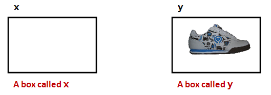
Each box has a unique name:
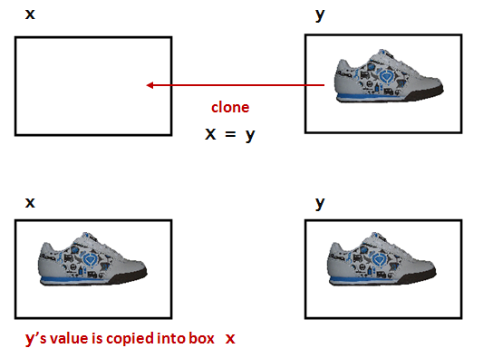
There is a cloning process that works like
this:
The value inside one box is cloned.
The cloned value is placed inside another.
There is a strange shortcut notation to specify cloning:
Here, the = (equals sign)
does NOT mean "equals."
It has been repurposed to mean
"clone", "copy," or, in programming-language
jargon, "assign".
How to say it: "x is assigned the value in y".
Important: Remember, a box can hold only one value at a time.
The technical term for our informal "box" is variable.
4.1 Integer variables
We'll now start working with "boxes" (variables) that hold
integers (whole numbers like 3, 17, 2097, but not numbers
like 3.141).
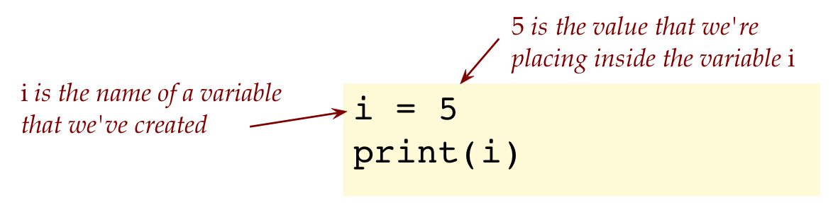
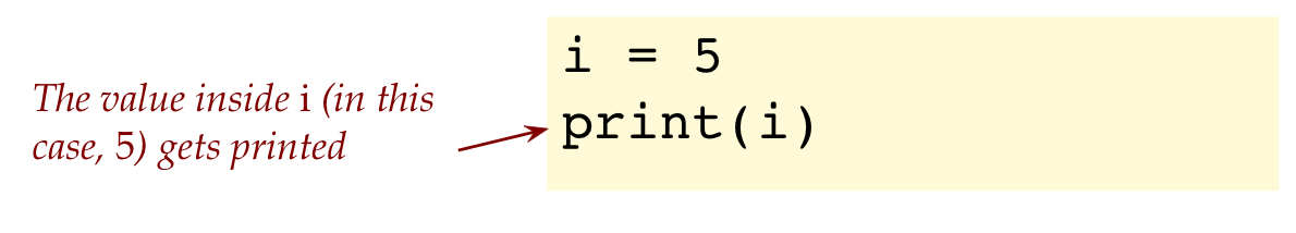
Consider this program:
i = 5
print(i)
4.1 Exercise:
Type up the program in
my_variable_example.py.
Also save the file so that it can be submitted
(Remember: you need to save the appropriate files for every
such "type up" exercise). What does it print?
Report what you see in
module4.pdf.
Now let's examine key parts of this program:
First, i is the name of a "box" (of sorts).
The term used for "box" is variable.
⇒ i is a variable.
To put something in a variable, we use assignment
⇒ with the repurposed = (equals) sign.
When we print a variable, what gets printed is its value.
⇒ Thus, the number 5 gets printed
Important: What you see on printed out is
the number 5
and NOT the letter i
Thus when you see
print(i)
you should think:
"Hmmm, the print function is going to print the contents
of variable i".
"I wonder what's inside i?"
"Let me look in the program to see what was the most recent value
that got written into i".
For example:
i = 5
i = 3
print(i)
4.2 Exercise:
Type up the above in
my_variable_example2.py
and confirm that 3 is what gets printed.
By way of explanation:
4.3 Exercise:
Is it possible to not have a value in a variable? Consider
this program:
i
print(i)
Type up the program in
my_variable_example3.py
What is the error?
Answer in module4.pdf.
(Remember, non-coding questions are to be answered in your module pdf,
in this case: module4.pdf.)
Thus: when you make a variable, you need to put something in it.
Next, let's look at assignment between variables:
This is the analogue of cloning between "boxes".
Consider this program:
i = 5
j = i     # The value in i gets copied into j
print(j)  # Prints 5
We say, in short, "i is assigned to j".
Notice: we've used comments above to annotate and explain.
We'll do this often, knowing that comments are not executed.
4.4 Exercise:
Consider this program:
i = 5
j = i
print(j)
print(i)   # Did i lose its value?
Type up the program in
my_variable_example4.py
and report what gets printed
in module4.pdf.
The above example illustrates that the value in
i
gets copied into the variable
j,
which means that the value 5 is still in
the variable
i.
4.5 Exercise:
Consider this program:
i = 5
j = i
k = j
print(k)
Try to identify the output of this program just by mental execution.
Type up the program in
my_variable_example5.py
and confirm.
4.6 Exercise:
Consider this program:
i = 5
j = i
i = 0
k = j
j = 0
print(k)
Try to identify the output of this program just by mental execution.
Type up the program in
my_variable_example6.py
and confirm.
Note that a copied value does not change if the original is changed:
For example, consider:
i = 5
j = i      # j now has 5
i = 0      # We changed i here
print(j)   # j still has 5
Here's the line-by-line execution:
The first line puts the value 5 in variable i.
The second line copies the value in i (which is 5)
into j. So j will have the value 5 as well.
The third line replaces the value 5 with value 0.
j still has 5, so the fourth line will print 5.
Note:
0 is an actual value, and is not "no value" or "nothing".
4.7 Video:
4.8 Exercise:
Type up
the following lines of code in
my_variable_example7.py:
i = 5
j = 6

# Add code between here

# and here.

print(i)   # should print 6
print(j)   # should print 5
Add some lines of code with the objective of swapping the
values in variables i and j. You will need a third variable to
be used as a holding place. Thus, without directly assigning the
number 5 to j or the number 6 to i, write code using a third
variable to achieve the desired swapping of values.
4.9 Video:
4.2 Integer operators
Let's examine the familiar arithmetic operators+, -, *, /
Addition: +
Subtraction: -
Multiplication: *
Division: /
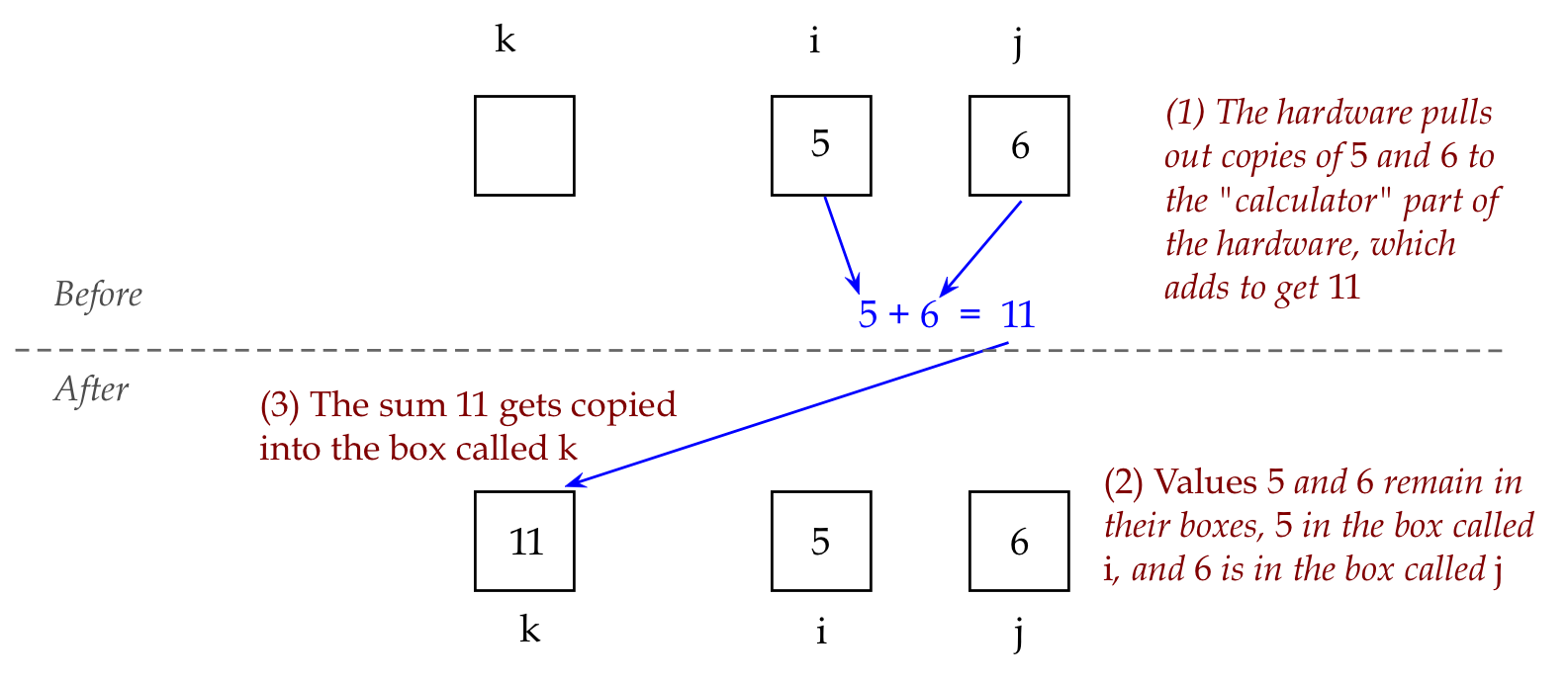
Consider this example with addition:
i = 5
j = 6
k = i + j
print(k)
What happens during execution:
The values in i and j
are added.
The resulting value goes into
variable k.
A long-ish way of saying this aloud:
⇒
"k is assigned the sum of the values of
i and j"
A shorter way:
⇒
"k is assigned i plus j"
Here's an example with multiplication and division:
i = 5
j = 6
k = i * j
print(k)      # prints 30
m = i / j
print(m)      # what does this print?
n = i // j
print(n)      # what does this print?
4.10 Exercise:
Type up the above in
my_variable_example8.py.
What is the value of n printed? Change i to 21. What is the value of n printed?
Answer in module4.pdf.
Submit your code with i set to 5.
Integer division:
In math, we learned that 1/4 = 0.25 and 21/6 = 3.5.
This remains true in Python when we do something like
      i = 21
      j = 6
      m = i / j
On the other hand, if we wish to perform
integer division, we can use the
integer division operator:
      i = 21
      j = 6
      m = i // j
That is, the result is truncated down to the
nearest integer.
Example: 3 // 2 becomes 1 because 1.5 gets truncated to 1.
Example: 15 // 4 becomes 3 because 3.75 gets truncated to 3.
Integer division is useful when we want to do integer
arithmetic.
4.3 Expressions and operator-precedence
Consider the following program:
i = 5
j = 6
k = i*j - (i+1)*(j-1)
print(k)
4.11 Exercise:
Type up the above program in
my_expression_example.py
What does it print?
Answer in module4.pdf.
About expressions:
An expression combines constants (like 1, above), and
variables using operators.
Example:
i*j - (i+1)*(j-1).
The above expression is really equivalent to:
(i*j) - ((i+1) * (j-1)).
Here, we added some clarifying parentheses.
Operator precedence allows us to reduce the
number of clarifying parentheses.
Python precedence follows standard precedence in math:
/, *, +, -.
You might remember the precedence via the acronyms
BODMAS or PEMDAS. (Look it up.)
The above expression is NOT the same as:
i*j - i+1*j-1.
Also, note the change of whitespace:
We could have written
k = i * j - (i + 1) * (j - 1).
But
k = i*j - (i+1)*(j-1).
is easier to read.
Let's dive a bit deeper into precedence and do some examples:
We'll use the four operators: add or +, subtraction or -,
multiplication or *, and division or /.
We'll use plain ol' numbers to illustrate.
Note: The key to working them out is to use extra
parentheses in the right way.
The PEMDAS rule:
First apply Parentheses, then Exponents, then
Multiplication and Division, and then Addition and Subtraction.
Example: 3 + 2*4
Here, we apply 2*4 to give 8
Then do 3 + 8 to give 11.
Applying extra parenthesis to 3 + (2*4) makes it clear.
Example: 3*(24/3-2*3)
First, work out what's inside the parens (the P of PEMDAS):
Do div to 24/3 and mult to 2*3 to get (8 - 6)
This gives (2)
Now go out and see that we need to do 3*(2)
Which gives 6.
Using extra parens and spacing makes it clear:
3 * ( (24/3) - (2*3) )
Example: 1 + ( (4 - 1) * 8) / 6
Do the innermost parens first: (4 -1) = 3
Which results in 1 + (3 * 8) / 6
Then the next parens to give: 1 + 24/6
Then the D in PEMDAS: 1 + 4
Result: 5
4.12 Exercise:
What does the expression i*j - i+1*j-1
evaluate to when i=7 and j=3?
Answer in module4.pdf.
4.13 Video:
4.4 More about expressions and assignment
The remainder operator:
The expression 10 % 3 is "the remainder when 10 is divided by 3".
Thus 10 % 3 is 1.
Similarly 11 % 4 is 3.
The remainder operator is sometimes called modulo,
as in "ten modulo 3 is 1"
Consider this example:
i = 14
j = -6
k = i % (-j)
print(k)
4.14 Exercise:
Can you mentally execute and identify what's printed?
Type up the above in
my_expression_example2.py
to confirm. Report the value in
module4.pdf
One way to know whether one number cleanly divides another
is to apply the
% (remainder)
operator.
Consider this program:
j = 10
for i in range(1, j):
    k = j % i
    print(k)
4.15 Exercise:
Can you mentally execute and identify what's printed?
Type up the above in
my_expression_example3.py
to confirm. Then change j to 11 and run the program.
Report the output in each case in
module4.pdf
When submitting the code, leave j as 11.
Note:
In the above exercise we systematically obtained the
remainder when dividing 10 (the value of j) by every possible
number less than 10.
Whenever the output is 0 in some iteration, we know 10 % i is 0
for that iteration.
This means i divides 10 cleanly (with no remainder).
For example 10 % 5 is 0.
Whenever a number j has nothing less than j that divides j
cleanly, the number is called a prime number.
Examples of prime numbers: 7 and 11.
Examples of non-prime numbers: 10 and 15
The notion of a prime number may seem like an esoteric
topic, suitable for a dinner conversation with mathematicians.
But it turns out to have immense practical value: much of
cryptography is based on properties of numbers that can
be cleanly divided by only two prime numbers.
4.16 Video:
Now we'll look at a strange (initially) but very useful type of
assignment:
Consider this program:
i = 8
i = i + i/2
print(i)
Prior to evaluating the expression, i has value 8.
On the right side, the current value of i is used
to evaluate the expression.
⇒ Thus, the expression evaluates to (8 + 8/2) = 12.
This evaluated value then goes into variable i.
⇒ After the assignment, i has the value 12.
Let's use this to compute the sum of numbers from 0 to 10:
s = 0
for i in range(0, 11):
    s = s + i
print(s)
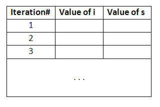
4.17 Exercise:
Trace the changing values of
s in the above program
using the following kind of table:
Write up the table in
module4.pdf.
Note: in this and other tracing exercises involving a table,
you can simply draw the table by hand and include a picture.
(That is, you don't have to spend time on making tables inside Word.)
Consider this program:
N = 5
s = 0
for i in range(1, N+1):
    s = s + (2*i - 1)
print(s)
The program prints the sum of the first N odd numbers.
Recall from earlier that as i goes through 1, 2, 3, ...
(2*i-1) evaluates as successive odd numbers 1, 3, 5, ...
4.18 Exercise:
Trace (in
module4.pdf)
the values of i and
s
in the program above.
Then, in
my_expression_example4.py,
edit the code to create an outer loop that varies N from
1 to 10. That is, make N a new for-loop variable that
ranges between 1 and 10 (inclusive), and ensure that you properly indent
the inner (nested) loop that uses i.
What pattern do you observe in the output?
4.19 Video:
4.5 Problem solving and pseudocode
Suppose we were given the following problem:
write a program to print the first N odd numbers.
We'll solve it in the following steps:
First, let's sketch out a "program-like" outline (not a real program):
       N = 10
       for i ranging from 1 to N:
           Calculate the i-th odd number
           Print it
This kind of rough outline is called pseudocode
⇒ We're meant to do this on paper, prior to programming.
Pseudocode looks a little like code, but is half-English.
For any given i, the i-th odd number is:
2*i - 1.
Now let's put this together into a program:
N = 10
for i in range(1, N+1):
    k = (2*i - 1)
    print(k)
4.20 Exercise:
Trace (in module4.pdf)
the values of i and
k
in the program above. This is what you should be able to do
mentally during mental execution.
4.6 A problem-solving example with variables and nested for-loops
We'll solve the following problem:
for any given n, compute
1 + 21 + 22
+ 23 + ... + 2n
That is, the sum of consecutive powers of 2.
As a first step, let's see if we can use a loop to
compute a single power of 2:
Suppose we wish to compute 2k for some
k.
We know that
2k
= 2*2*2 ... *2 (k times)
Thus, what we could is:
Start with p = 1
Multiply by 2: p = p * 2
Multiple that result by 2: p = p * 2
... etc
In pseudocode:
       p = 1
       for i ranging from 1 to k:
          p = p * 2
Let's put this into code and test:
k = 10
p = 1
for i in range(1, k+1):
    p = p * 2
print(p)
4.21 Exercise:
Trace the changing values of p
in the above program using a table
(in module4.pdf).
Then, type up the above program in
my_powerof2.py
to confirm.
4.22 Video:
Next, let's look at pseudocode for the sum of powers (our
original problem):
       s = 1
       for k ranging from 1 to n:
           Compute k-th power of 2
           Accumulate in s
       Print s
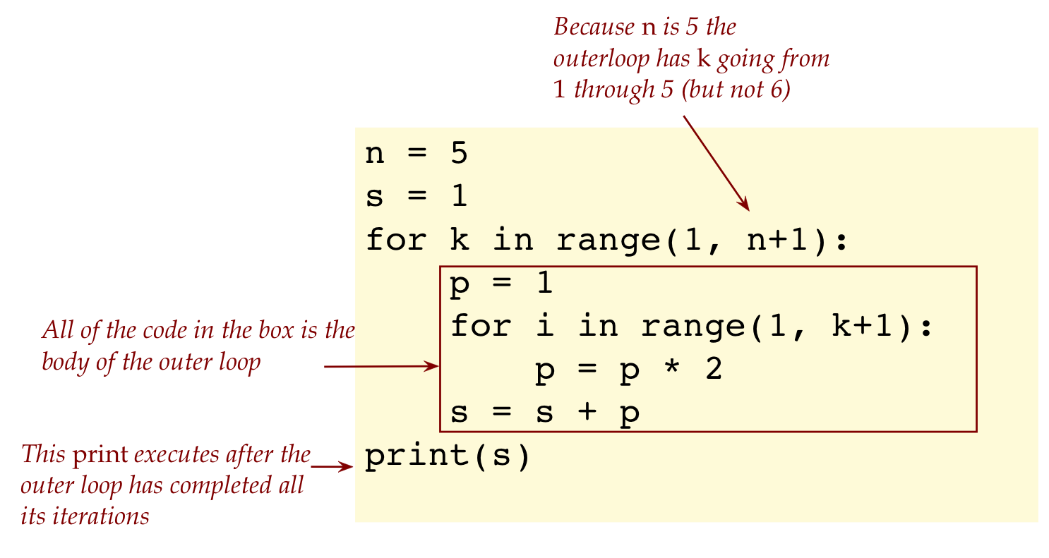
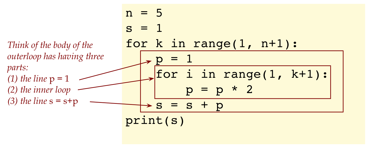
Now, let's put this all together:
n = 5
s = 1
for k in range(1, n+1):
    p = 1
    for i in range(1, k+1):
        p = p * 2
    s = s + p
print(s)
Let's point out a few things.
First, let's have our eyes look over the outer-loop and not
focus on the details of the inner loop:
Now look inside the body of the outerloop:
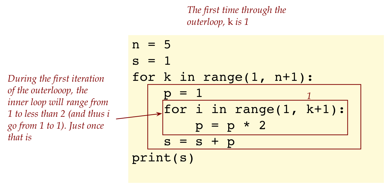
Try to get a feel for how it executes by looking at the
first iteration of the outerloop:
4.23 Exercise:
Make a table with columns labeled k, i, p
and s and trace the program, filling
in the table step-by-step
(in module4.pdf).
4.24 Video:
4.25 Exercise:
Try a few other values of n, e.g., n=3
or n=4. Try to guess the mathematical formula for
1 + 21 + 22
+ 23 + ... + 2n.
(in
module4.pdf)
Hint: add 1 to the sum-of-powers of 2.
4.7 Shortcut operators
Recall the integer-sum program:
s = 0
for i in range(0, 11):
    s = s + i
print(s)
We can write this using the "shortcut addition" operator += as follows:
s = 0
for i in range(0, 11):
    s += i
print(s)
Thus,
s += i is the same as
s = s + i
One can read
s += i
as "add i to what's already in s, and store the result in s".
This can be applied to the other operators as well:
       s -= i         # Same as s = s - i
       p *= 2         # Same as p = p * 2
       d /= 2         # Same as d = d / 2
4.26 Exercise:
In
my_sum_powerof2.py
rewrite the example code that computes the sum of power of 2,
using shortcut operators where possible.
4.8 When things go wrong
As you might imagine, there are many ways to inadvertently
create errors.
In each case below, first try to identify the error just
by reading. Then, type up the program to confirm.
4.27 Exercise:
What is the error in this program?
i = j
j = 4
print(i)
Type it up in
error1.py
to confirm.
4.28 Exercise:
What is the error in this program?
i = 4
j = 3
k = ( (i + j) * (i - j) / 2
print(k)
Type it up in
error2.py
to confirm.
We'll now see a different kind of error:
n = 5
for i in range(1, n+1):
    k = n / (n - i)
    print(k)
4.29 Exercise:
Type it up in
error3.py
and see. Then trace through the program at each iteration
in
module4.pdf.
The above is an example of a runtime error:
The code itself is correctly written in that there
are no issues with breaking the rules of the language.
However, when i is 0, you can't divide by 0.
This causes a runtime error, meaning the program
runs fine until the particular occurence of divide-by-zero.
4.9 Python files vs module pdf
Important:
By now it should be clear what you type into
a Python file (ends with
.py)
verses what goes into your module pdf.
Code goes into the specified Python file
(example:
error3.py)
and all other answers go into your
module pdf
(numbered by module#, such as:
module4.pdf).
Your module pdf (a single pdf per module)
will have all the non-coding answers for a module.
Whereas, a module can have many different Python files.
Thus, in future modules, we will only specify
the Python filename with the understanding that you know
how to name your module pdf.
4.10 A peek at the future
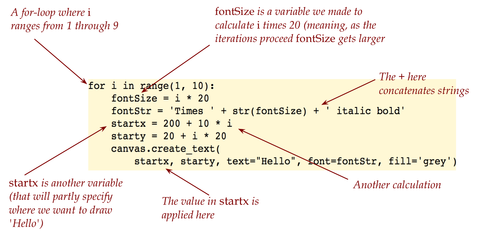
Let's now revisit some earlier code
(hello_gui.py)
and apply what've learned about integers, arithmetic, and for-loops:
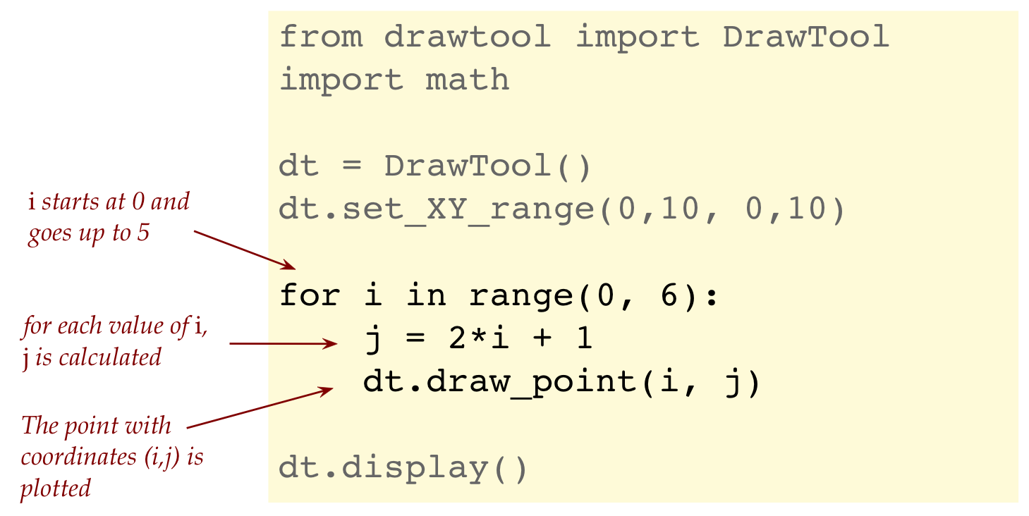
Next, consider this program that uses a for-loop to plot
points:
from drawtool import DrawTool
import math

dt = DrawTool()
dt.set_XY_range(0,10, 0,10)

for i in range(0, 6):
    j = 2*i + 1
    dt.draw_point(i, j)

dt.display()
4.30 Exercise:
Download drawtool.py
into your module4 folder. Then,
type up the above in
my_plot_points.py,
and run.
Let's point out:
Let's focus on the parts we recognize (the for-loop):
So, when i is 0, j is calculated as 1
This plots the point (0,1).
Then, when i is 1, j becomes 3, which results in the point (1,3).
... and so on.
The points are the dots shown in the plot.
When you downloaded
drawtool.py,
you downloaded another Python program into the same folder.
This is a program that provides drawing and plotting features.
We've used one of its features here (plotting points),
and will use
drawtool.py
again in the future.
Notice that the plotted points are along a straight line,
implying a linear relationship between i and j.
We will occasionally write programs that work with numbers
and quantitative concepts. As a result, we'll encounter mathematical
ideas in a different way, through programming.
4.11 Meta
Another in our series of occasional "meta" sections that will
step back from the material to comment on how we can learn better.
This was a loooong module with lots of exercises and details.
Let's review:
We introduced the all-important concept of a variable
along with the sense that there's a "place" in the computer
for each variable.
⇒
The "place" is really in the memory (also called RAM) of the computer.
Along with variables is the notion of assignment,
which means "copying the value in one variable into another variable".
Note: assignments are amongst the most common of statements
in everyday code.
When a variable is of a numeric type like integers, we also
need to go over basic operators and show examples.
Further complications arose when the operators have variations.
Since we were on the topic of integers, we took this
opportunity to learn how to do some number-crunching.
When we got to nested loops, it got tricky following the
values of variables through multiple nested loops.
So, if you felt a bit overwhelmed, that's perfectly understandable.
If you have to go back to some of the material to review or try
some exercises again, that's fine. You're going to get better at this!