Exercise 1:
Download and execute QueueControl.java
to estimate the average waiting time per customer.
Some (unanswered) issues regarding the estimate:
- How many customers should one observe before we're sure we
have an accurate enough estimate?
- What is accurate enough? A few decimal places?
- Is it better to run a long simulation or take the average
across many simulation runs?
→ Would they give different results?
In this module, we want to understand what probability theory
can tell us about such estimates.
To look into this, we'll need some more background:
- How to reason about functions of random variables (rv's).
- How to reason about sequences of rv's.
- A new measure: variance.
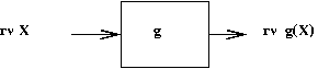
9.2 Functions of random variables
Recall our favorite example, the 3 coin flips (with \(\prob{H}=0.6\)):
Exercise 3:
Suppose that \(X\simm{Uniform}(0,1)\) and \(g(X)=X^2\).
Modify UniformExample.java
to estimate the pdf of \(g(X)\) and its average value.
You will also need RandTool.java
and DensityHistogram.java.
What do you notice about the average value of \(g(X)\) compared
with the average value of \(X\)?
One obvious question is: do any rv's retain the form of their
distribution through simple transformations?
Exercise 4:
Suppose \(X\simm{Uniform}(0,1)\) and
\(Y=3X\).
What is the range of \(Y\)?
Modify UniformExample3.java
and estimate the density of \(Y\).
Some distributions maintain their "distribution type" (with
different parameters):
- If \(X\simm{Uniform}(0,1)\), then
\(aX+b\simm{Uniform}(b,b+a)\)
- If \(X\simm{N}(0,1)\), then
\(aX+b\simm{N}(b,a^2)\)
Expectation of a function of a rv:
- We've already seen the discrete case: if \(g(X)\) is a
function of discrete rv \(X\):
$$
\expt{g(X)} \eql \sum_k g(k) \prob{X=k}
$$
- For the continuous case, the analog is:
$$
\expt{g(X)} \eql \int_{-\infty}^{\infty} g(x) f(x)
$$
- It's important to get some intuitive sense of what this
means:
- Think of the discrete case as a weighted sum
\(\Rightarrow\) Each \(g(k)\) weighted against its corresponding
\(\prob{X=k}\) value.
- In the continuous case, break it up into small intervals
\(\Rightarrow\) \(g(x_i)\) is the value of \(g( )\) in the
\(i\)-th interval, and \(f(x_i)*\delta\) is the
probability (for that interval).
\(\Rightarrow\)
\(\sum_i g(x_i) f(x_i) \delta\) is also a weighted sum.
\(\Rightarrow\)
In the limit, this becomes the integral
\(\int_{-\infty}^{\infty} g(x) f(x) \)
Exercise 5:
Suppose \(X\) is the 3-coin flip rv (with \(\prob{H}=0.6\))
and \(g(x)\) is the function \(g(x)=(x-1.8)^2\).
Work out \(\expt{g(X)}\) by hand.
Then estimate the average value of the rv \(g(X)\)
by adding code to CoinExample.java.
(You'll also need Coin.java).
Exercise 6:
Suppose \(X\simm{Uniform}(0,1)\)
and \(g(x)\) is the function \(g(x)=(x-0.5)^2\).
Work out \(\expt{g(X)}\) by hand.
Then estimate the average value of the rv \(g(X)\)
by adding code to UniformExample4.java.
9.3 Variance
Variance is what we get for a special case of the function \(g( )\) above:
- A formal definition looks like this:
\(\mbox{var}[X] = \expt{(X - \expt{X})^2}\)
- This is a little confusing, so let's tease out the meaning.
- First, recall that \(\expt{X}\) is a number. We'll give
this a symbol:
\(\mu = \expt{X}\)
- Assume we have already calculated this value.
- Next, define the function \(g(x) = (x - \mu)^2\).
- We know how to compute \(\expt{g(X)}\) for any
function \(g(x)\)
\(\Rightarrow\) We simply compute \(\expt{g(X)}\) for the particular
function \(g(x) = (x - \mu)^2\).
- Define variance as
\(\mbox{var}[X] = \expt{g(X)}\) for the particular
function \(g(x) = (x - \mu)^2\).
- Variance is a measure of "spread"
\(\Rightarrow\) Generally, the wider (more spread out) a distribution, the
larger the variance.
- Note: (1) This is not always true, and (2) there are other
measures of spread.
- The variance is sometimes presented as its square-root,
called the standard deviation
\(\mbox{std}[X] = \sqrt{\mbox{var}[X]}\).
Exercise 7:
Suppose \(X\) is a rv with range \({9,11}\) and pmf
\(\prob{X=9} = 0.5\)
\(\prob{X=11} = 0.5\)
and \(Y\) is a rv with range \({8,12}\) and pmf
\(\prob{Y=8} = 0.5\)
\(\prob{Y=12} = 0.5\)
and \(Z\) is a rv with range \({8,10,12}\) and pmf
\(\prob{Z=8} = 0.1\)
\(\prob{Z=10} = 0.8\)
\(\prob{Z=12} = 0.1\)
Compute \(\mbox{var}[X], \mbox{var}[Y]\) and \(\mbox{var}[Z]\).
9.4 Reasoning about multiple rv's
Most real-world applications have more than one rv of interest
in an application
e.g,, in the Queueing application we could be interested in
both the waiting time and the service time at Queue 0.
A simple example with two rv's \(X\) and \(Y\):

- Consider points generated on the plane
\(\Rightarrow\) Each point is an \((x,y)\) pair.
- When the points are randomly generated,
\(\Rightarrow\) let rv \(X\) denote the x-value, and rv \(Y\) denote
the y-value.
Exercise 8:
Download and execute
PointGeneratorExample.java.
You will also need
PointGenerator.java
and PointDisplay.java.
Increase the number of points to 1000. Can you guess the distribution
of \(X\)? Of \(Y\)?
Exercise 9:
Download and modify
PointGeneratorExample2.java
to display density histograms for \(X\) and \(Y\).
Distributions for \(X\) and \(Y\):
- Note that both \(X\) and \(Y\) are continuous rv's above.
\(\Rightarrow\) Both will have pdfs
- Even though both \(X\) and \(Y\) occur together,
each has its own range.
\(\Rightarrow\) Each has its own pdf, as was evident from the density histogram.
- In some books, such separate distributions for
jointly-occuring rv's are called marginal distributions.
Next, let's consider dependence (or independence):
- Recall the definition used with events:
Events \(A\) and \(B\) are independent if \(\prob{A | B} = \prob{A}\).
- As we will see, it is easy to extend this definition to rv's.
- First, let's consider the point example:
- Suppose we consider the events \(X \in [3,4]\), and
\(Y \in [5,7]\).
- Let's ask whether \(\prob{Y\in [5,7] \;|\; X\in [3,4]}
= \prob{Y\in [5,7]}\).
Exercise 10:
Download and examine
PointGeneratorExample3.java.
The first part of the code estimates \(\prob{Y\in [5,7]}\).
Add code below to estimate
\(\prob{Y\in [5,7] \;|\; X\in [3,4]}\).
Are these events independent?
Exercise 11:
Now change the method randomPoint() to
randomPoint2() and see what you get.
Are the two events independent?
Independence for rv's:
- We say that rv's \(X\) and \(Y\) are independent
if for all events \(A\) and \(B\):
\(\prob{Y\in B \;|\; X\in A} = \prob{Y\in B}\).
- How do we know whether two rv's are actually independent?
Should we try all possible events \(A\) and \(B\)?
- In practice:
- We either assume independence (for separate, repeatable experiments).
- Or we estimate the dependence.
The idea of a conditional distribution:
- Recall the conditional probability
\(\prob{Y\in [5,7] \;|\; X\in [3,4]}\).
- Let's use the event \(X\in A\) to denote
an event like \(X\in [3,4]\).
- For any interval \([a,b]\) one could obtain
\(\prob{Y\in [a,b] \;|\; X\in A}\).
- In particular, suppose we divide the range of \(Y\) into
many little intervals
\([0,\delta], [\delta,2\delta], [2\delta,3\delta], ...\)
- For every such interval, one could evaluate
\(\prob{Yε[i\delta,(i+1)\delta] \;|\; X\in A}\).
\(\Rightarrow\) In effect, this is a histogram of \(Y\) given
\(X\in A\).
- One can turn this into a density histogram.
- In the limit as \(\delta \to 0\), this becomes a pdf.
\(\Rightarrow\) It becomes the conditional pdf of
\(Y\) given \(X\in A\).
Exercise 12:
Download and examine
PointGeneratorExample4.java.
You should see two histograms being computed: one without the
conditioning, and one with. Execute and compare.
What do you get when using
randomPoint2()?
Another definition of independence:
- Rv's \(X\) and \(Y\) are independent if for
every event \(A\), the conditional distribution of \(Y\)
given \(X\in A\) is the same as the distribution of \(Y\).
Discrete rv's
- All our discussion has centered on continuous rv's.
Does this work for discrete rv's?
\(\Rightarrow\) Yes, except that we use pmfs instead of pdfs.
- Consider this game: I roll two dice - if the same
number shows up on both, I win.
- Let's write a program to estimate the odds of winning:
(source file)
        double numTrials = 100000;
        double numSuccesses = 0;
        Dice dice = new Dice ();
        for (int n=0; n<numTrials; n++) {
            dice.roll ();
            if ( dice.first() == dice.second() ) {   // Win?
                numSuccesses ++;                     // Count # wins.
            }
        }
        double prob = numSuccesses /  numTrials;     // Estimate.
        System.out.println ("\prob{win] = " + prob);
Exercise 13:
Without executing the above program, what is the probability
of winning?
Download DiceExample.java
and confirm your answer. You will also need
Dice.java
Exercise 14:
Next replace
Dice.java
with
DodgyDice.java
and see what you get.
- Let's analyse the second pair of dice, starting with
a histogram.
Let \(X\) denote the outcome of the first die, and
\(Y\) the outcome of the second.
Exercise 15:
Modify DiceExample3.java
to obtain a histogram for \(Y\). Does this reveal anything
suspicious?
- Next, let us estimate the conditional pmf
\(\prob{Y=k \;|\; X=1}\) and see if that reveals anything.
Exercise 16:
Modify DiceExample4.java
to obtain a histogram for \(Y\) given \(X=1\).
What should the histogram look like for fair dice?
- Thus, we see that essentially the same reasoning applies
to discrete rv's.
9.5 Sums and functions of multiple rv's
Functions of multiple rv's:
- If \(h(x,y)\) is a function of two variables and
\(X, Y\) are two rv's
\(\Rightarrow\) \(h(X,Y)\) is a rv.
- Example: \(h(x,y) = x+y\),
where \(X\simm{Uniform}(0,1)\),
and \(Y\simm{Uniform}(0,1)\)
Then, \(h(X,Y)\) is a rv
Exercise 17:
What is the range of \(h(X,Y)\)?
Do you expect the rv \(h(X,Y)\) to have a uniform distribution?
Modify UniformExample2.java
and find out. Is the average what you expected?
Do sums of rv's have the same distribution as the addends?
- Generally, sums rarely maintain distribution form.
- The Normal distribution is an exception:
If \(X\simm{N}(\mu_1, \sigma_1^2)\)
and
\(Y\simm{N}(\mu_2, \sigma_2^2)\)
then
\(X+Y\simm{N}(\mu_1+\mu_2,
\sigma_1^2 + \sigma_2^2 )\)
Sometimes a sum of one type of rv has a well-known distribution
(of another type)
- Example: consider flipping a coin \(n\) times.
- Let \(X_i\) be the Bernoulli rv
representing the \(i\)-th flip:
\(\Rightarrow\) \(X_i = 1\) if \(i\)-th flip was "heads", and \(0\) otherwise.
- We'll assume the successive flips are all independent.
- Define the sum rv
\(S_n = X_1 + X_2 + \ldots + X_n\)
- If \(X_i \simm{Bernoulli}(p)\), then
\(S_n \simm{Binomial}(n,p)\).
9.6 The estimation problem
Let's look at the most intuitive type of estimation:
- Suppose we observe the (numeric) outcome of an experiment
\(\Rightarrow\) we want to compute the average (mean) value.
- For example:
     Algorithm: estimateMean (N)
     Input: number of trials
     1.   total = 0
     2.   for n=1 to N
     3.       x = result of experiment
     4.       total = total + x
     5.   endfor
     6.   return total/N
- A Java implementation:
(source file)
        double numTrials = 100000;
        double total = 0;
        for (int n=0; n<numTrials; n++) {
            // Perform the experiment and observe the value.
            double x = Experiment.getValue ();
            // Record the total so far.
            total = total + x;
        }
        // Compute average at the end.
        double avg = total / numTrials;
        System.out.println ("Mean: " + avg);
- This simple age-old procedure raises some questions:
- Exactly how many trials should one perform?
- What is the theoretically correct value for the mean?
\(\Rightarrow\) What is the relationship between what's estimated and the
theory developed thus far?
Before looking deeper, consider other types of estimation problems:
- We might be interested in estimating a distribution:
\(\Rightarrow\) pmf for a discrete rv, pdf for a continuous rv
- We might be interested in measuring "spread" or
some other such characteristic of the data.
- The earlier, most basic type of estimation (using the mean)
is called point estimation.
Let's place point estimation in a theoretical framework:
- Suppose we have an experiment and perform \(n\) trials.
- Let \(X_i\) be the outcome of the \(i\)-th trial.
- Define the sum rv
\(S_n = X_1 + X_2 + \ldots + X_n\)
- Then, the average that we print is
\(\frac{S_n}{n}\).
- We can now frame one of the questions more carefully: what is
$$
\lim_{n\to\infty} \frac{S_n}{n}
$$
Does this converge to a number? Some other kind of
mathematical object?
- We sense that this converges to a number. Let's assume (for
a moment)
$$
\lim_{n\to\infty} \frac{S_n}{n} \eql \nu
$$
where \(\nu\) is a number.
- A second question relates to a fixed number of samples
\(n\): what is the distribution of \(\frac{S_n}{n}\)?
\(\Rightarrow\) If we know this distribution, we could ask what is
\(\prob{\frac{S_n}{n} \gt \nu + \delta}\)?
\(\Rightarrow\) In other words, what is the probability that our estimate
\(\frac{S_n}{n}\) will be "off" by a distance \(\delta\)?
- Unfortunately, these questions look hard:
- We don't know anything (yet) about limits for rv's.
- We've seen that the distribution for a sum is known
for only a few distributions.
\(\Rightarrow\) In a real-world application, we won't even know the distribution!
- Fortunately, there are two powerful results (developed over
200 years) in probability theory, which we'll state informally:
- The Law of Large Numbers:
If the \(X_i\)'s are independent (and
all have the same distribution)
$$
\lim_{n\to\infty} \frac{S_n}{n} \eql \expt{X_1}
$$
- The Central Limit Theorem: the distribution of the rv
\(\frac{S_n}{\sqrt{n}} \) is approximately Normal.
- What are the implications?
- From the Law of Large Numbers:
- We know that \(\frac{S_n}{n}\) converges to
something - a number.
- Even better, it converges to a special number
\(\expt{X_i}\) that's
computed based on the distribution (pmf, pdf) of any one
of the rv's \(X_i\).
- It's reassuring to know that the limit corresponds to our
intuition about the expected value.
- The CLT is more significant:
- If we can approximate the distribution of
\(\frac{S_n}{n}\), we can compute probabilities
associated with \(\frac{S_n}{n}\).
\(\Rightarrow\) In particular, the probability that
\(\frac{S_n}{n}\) is "close enough" to the limit.
\(\Rightarrow\) If it isn't, we make \(n\) larger (more samples).
- Most importantly, the limit distribution of \(\frac{S_n}{n}\)
does not depend on the distribution of \(X_i\).
\(\Rightarrow\) \(X_i\) could be any distribution
(discrete or continuous).
9.7 Sequences of rv's
Let's return to our simple estimation problem:
- Recall, \(X_i\) is the outcome of the \(i\)-th
trial
and \(S_n = X_1 + X_2 + \ldots + X_n\)
- Then, our estimate with \(n\) samples is
\(\frac{S_n}{n}\).
- Now, for each \(n\), \(\frac{S_n}{n}\) is a random variable.
- Thus, the sequence
\(\frac{S_1}{1}, \frac{S_2}{2}, \frac{S_3}{3} \ldots \)
is a sequence of rv's.
- Let's look at a specific example: suppose we are estimating
the mean of a uniform distribution:
- In our experiment, samples come from a uniform generator.
- The rv \(X_i\) is the result of the \(i\)-th call.
- Some sample code:
(source file)
        double numTrials = 10;                // n=10
        double total = 0;
        for (int i=1; i<=;numTrials; i++) {   // Note: i starts from 1.
            double x = RandTool.uniform ();   // Xi = outcome of i-th call to uniform()
            total += x;
        }
        double avg = total / numTrials;       // Sn / n
                                              // = (X1 + ... + Xn) / n
        System.out.println ("Avg: " + avg);
Exercise 18:
Modify UniformMeanExample.java
to print out successive values of
\(\frac{S_1}{1}, \frac{S_2}{2}, \frac{S_3}{3} \ldots\).
Put these values into a Function and display.
The idea of a sample path or sample run:
- In the uniform example above, the generator started
with some seed.
- We will now change the seed and observe what happens:
(source file)
        // The first "run": set the seed to some value.
        RandTool.setSeed (1234);
        double total = 0;
        for (int i=1; i<=numTrials; i++) {
            double x = RandTool.uniform ();
            total += x;
            System.out.println ("i=" + i + "  S_i/i=" + (total/i));
        }
        double avg = total / numTrials;
        System.out.println ("Avg: " + avg);


        // The second "run": set the seed to some other value and repeat.
        RandTool.setSeed (4321);
        total = 0;
        for (int i=1; i<=numTrials; i++) {
            double x = RandTool.uniform ();
            total += x;
            System.out.println ("i=" + i + "  S_i/i=" + (total/i));
        }
        double avg = total / numTrials;
        System.out.println ("Avg: " + avg);
Exercise 19:
Modify UniformMeanExample2.java
to compare the output from each run.
Put \(\frac{S_1}{1}, \frac{S_2}{2}, \frac{S_3}{3} \ldots \)
values from the first run into one Function
object, and the values from the second run into a
second Function object. Display both together
using the Function.show (Function f1, Function f2) method.
- Clearly, each run or sample path is different.
\(\Rightarrow\) What does this say about the sequence
\(\frac{S_n}{n}\)?
\(\Rightarrow\) It is unlike a sequence of real numbers.
- Furthermore, consider this (artificial) sample path:
\(0.1, 0.2, 0.1, 0.2, 0.1, 0.2, ...\) (alternating 0.1 and 0.2)
\(\Rightarrow\) Although unlikely, it is certainly possible.
Exercise 20:
What does \(\frac{S_n}{n}\) converge to on this sample path?
- Thus, there are sample paths on which \(\frac{S_n}{n}\)
does not converge to 0.5.
We sense they are unlikely to occur, but can we say this rigorously in some way?
Limits of sequences of rv's:
- There are two types of limits to consider for a sequence of rv's:
- A sequence of rv's can converge to a number.
- A sequence of rv's can converge to another rv.
- Let's consider the first kind.
\(\Rightarrow\) There are several ways in which we can say a sequence or rv's
converges to a number.
- We'll consider these next. For each of these we'll, in
general, ask whether a sequence rv's
\(Y_n\) converges to a number \(\nu\).
Convergence in probability:
- The formal definition:
the sequence \(Y_n\) converges to \(\nu\)
in probability if
for any \(\delta \gt 0\)
$$
\lim_{n\to\infty} \prob{|Y_n - \nu| \gt \delta} \eql 0
$$
- What is the definition saying?
- You pick some tiny \(\delta \gt 0\), e.g., \(\delta =
0.0001\)
- Then, for any \(n\), we could (in theory) compute
\(\prob{|Y_n - \nu| \gt \delta}\).
- Let \(y_n = \prob{|Y_n - \nu| \gt \delta}\).
- Now, the numbers \(y_1, y_2, \ldots, ...\)
are a sequence of real numbers.
- The definition requires that the sequence \(y_1, y_2, \ldots, ...\)
converges to zero.
- Intuitively, the probability that "the rv
\(Y_n\) differs from \(\nu\)"
gets smaller as \(n\) grows large.
- Convergence in probability is sometimes called weak convergence.
Convergence in mean-square:
- An alternative definition is to look at the rv
\(Y_n - \nu\) and its expectation
\(\expt{Y_n - \nu}\)
- Intuitively, if it's true that \(Y_n \to
\nu\), then \(\expt{Y_n - \nu} \to 0\) should be true.
- Indeed, it should also be true that
\(\expt{(Y_n - \nu)^2} \to 0\).
\(\Rightarrow\) This is the preferred definition.
- More formally,
the sequence \(Y_n\) converges to \(\nu\) in
mean-square if the sequence of real numbers
\(\expt{(Y_n - \nu)^2} \to 0\).
Exercise 21:
Can you construct an artifical sequence of rv's
\(Y_n\) such that \(\expt{Y_n - \nu} \to 0\)
but that \(Y_n\) clearly doesn't converge to any number?
[Hint: create a sequence such that
\(\expt{Y_n - \nu} = 0\) for all \(n\)].
Convergence almost-surely:
- This is the most interesting kind, but is harder to understand.
- First, let's go back to our uniform example:
- Consider the output of the uniform generator:
        double total = 0;
        for (int i=1; i<=numTrials; i++) {
            double x = RandTool.uniform ();   // X_i = outcome of i-th call to uniform()
            total += x;
            // Print Xi for each i.
            System.out.println ("i=" + i + " x=" + x);
        }
- Here's a sample from 10 calls to the generator:
       i=1  x=0.5053
       i=2  x=0.2366
       i=3  x=0.6297
       i=4  x=0.7279
       i=5  x=0.4147
       i=6  x=0.8428
       i=7  x=0.7029
       i=8  x=0.4018
       i=9  x=0.8628
       i=10 x=0.3155
- Let's also print out the running average
\(\frac{S_1}{1}, \frac{S_2}{2}, \frac{S_3}{3} \ldots \):
        double total = 0;
        for (int i=1; i<=numTrials; i++) {
            double x = RandTool.uniform ();   // X_i = outcome of i-th call to uniform()
            total += x;
            // Print Xi for each i.
            System.out.println ("i=" + i + " x=" + x + "  S_i/i=" + (total/i)););
        }
- Sample output:
       i=1  x=0.5053  S_i/i=0.5053
       i=2  x=0.2366  S_i/i=0.3710
       i=3  x=0.6297  S_i/i=0.4572
       i=4  x=0.7279  S_i/i=0.5249
       i=5  x=0.4147  S_i/i=0.5028
       i=6  x=0.8428  S_i/i=0.5595
       i=7  x=0.7029  S_i/i=0.5800
       i=8  x=0.4018  S_i/i=0.5577
       i=9  x=0.8628  S_i/i=0.5916
       i=10 x=0.3155  S_i/i=0.5640
- Thus, it looks like the running average will eventually
converge to 0.5.
- However, what if the uniform generator produced this sequence?
       i=1  x=0.1
       i=2  x=0.2
       i=3  x=0.1
       i=4  x=0.2
       i=5  x=0.1
       i=6  x=0.2
       i=7  x=0.1
       i=8  x=0.2
       i=9  x=0.1
       i=10 x=0.2
Clearly, on this sequence, the average does NOT converge to 0.5
- Sure, it's unlikely, but can we say it can't happen?
- Now, if we want to consider the limiting behavior of a
sequence of rv's, we need to consider complete sample paths.
- For the uniform generator, what does the set of all
possible sample paths look like?
- That set willcontain the sample path \(0.1, 0.2, 0.1, 0.2, ...\)
- It will also contain \(0.5053, 0.2366, 0.6297, ... \) (the
first output from the generator).
- In fact, it will consist of every conceivable path.
- Let \(\Omega\) denote the set of all sample paths.
- Let \(\omega\) denote a particular sample path in \(\Omega\).
- Then, on this sample path, either we get convergence to our
desired limit or not.
- For example, if \(\omega\) is the path \(0.1, 0.2,
0.1, 0.2, ...\), we don't get convergence to 0.5 (the desired limit).
- Next, let's group the sample paths into two sets:
- \(\Omega_A\) = set of all sample paths
on which we do get the desired limit.
\(\Rightarrow\) Note: \(\Omega_A\) is an event.
- \(\Omega_B = \Omega - \Omega_A\) =
the set of sample paths on which we do NOT get the desired result.
\(\Rightarrow\) Similarly, \(\Omega_B\) is an event.
- Then, a meaningful question is: what is \(\prob{\Omega_A}\)?
Or, equivalently, what is \(\prob{\Omega_B}\)?
- Note: \(\prob{\Omega} = 1\).
- OK, back to our sequence \(Y_n\) and its
supposed convergence to a number \(\nu\)
- Suppose we collect into \(\Omega_A\)
all sample paths on which it DOES converge to \(\nu\).
- Similarly \(\Omega_B\) = all sample paths on
which \(Y_n\) does NOT converge to \(\nu\).
- Now, finally, the definition: we say that
\(Y_n \to \nu\) almost-surely if
\(\prob{\Omega_A} = 1\).
- This type of convergence is also called strong convergence.
(There are other names too, e.g., convergence almost-everywhere).
- Whew!
Which definition should we prefer?
- What is known:
- Convergence-a.s. implies convergence in probability,
- Mean-square-convergence implies convergence in probability.
- There are (strange) counterexamples where convergence-a.s.
does not result in convergence-mean-square and vice-versa.
- These distinctions usually matter when you are in the
business of proving such results (advanced probability).
9.8 Law(s) of Large Numbers
Let's now return to our favorite sequence:
- The sequence \(\frac{S_n}{n}\) where
\(S_n = X_1 + X_2 + \ldots + X_n\)
and \(X_i\) is the outcome of the \(i\)-th trial
in an experiment.
- We wondered whether \(\frac{S_n}{n}\to \) any
real number.
- It can be shown that: \(\frac{S_n}{n}\to \expt{X_1}\)
in probability
\(\Rightarrow\) This is called the Weak Law of Large Numbers
- It can be shown that \(\frac{S_n}{n} \to \expt{X_1}\) almost-surely
\(\Rightarrow\) This is called the Strong Law of Large Numbers
- The former is easier to prove and requires fewer technical
conditions (like smoothness of distributions etc).
- The latter is conceptually deeper and took much longer to
develop.
What does all this mean?
- It means the natural, intuitive process of estimation has a firm
theoretical basis.
\(\Rightarrow\) The estimation procedure (taking the average) eventually does
convergence to the expected value.
- This is NOT true for other kinds of estimates, for
example: the geometric mean
\(G_n = (X_1 X_2 \ldots X_n)^{\frac{1}{n}}\)
or the harmonic mean
\(\frac{1}{H_n} = \frac{1}{n} (\frac{1}{X_1} + \frac{1}{X_2}
+ \ldots + \frac{1}{X_N}) \)
- Both the geometric and harmonic mean are alternative
measures of central tendency, and have some desirable
properties, but guaranteed convergence to the expected value is
not one of them.
9.9 The Central Limit Theorem and confidence intervals
We will now return to our estimation example with the uniform
distribution:
- Recall that \(\frac{S_n}{n}\) is our estimate of the mean.
- For a particular, fixed \(n\) (e.g., \(n=5\)),
\(\frac{S_5}{5}\) is a rv with some distribution.
- Consider a slight variation of the sequence:
\(S^\prime_n = (S_n - n 0.5)\)
- Clearly, because \(\frac{S_n}{n} \to 0.5\), it
must be that \(\frac{S^\prime_n}{n} \to 0\)
- Let us examine the rv \(\frac{S^\prime_n}{n}\)
by getting a histogram:
     Algorithm: histogramForS'n_over_n (n)
     Input: n, the fixed number of samples of Xi's.
     1.   for r=1 to numRuns
     2.       total = 0
     3.       for i=1 to n
     4.           x = uniform ()            // The i-th call produces \(Xi\).
     5.           total = total + x
     6.       endfor
     7.       avg = total / n               // avg = S_n / n
     8.       histogram.add (avg-0.5)       // S'_n / n
     9.   endfor
     10.  return histogram
- In Java, this looks like:
(source file)
        // We'll build a density-histogram in the range [-2,2] with 20 intervals.
        DensityHistogram hist = new DensityHistogram (-2,2,20);

        // Number of runs over which to collect samples of S_n/n
        double numRuns = 100000;

        for (int r=0; r<numRuns; r++) {

            double n = 5;
            double total = 0;
            for (int i=1; i<=n; i++) {
                double x = RandTool.uniform ();   // X_i = outcome of i-th call to uniform()
                total += x;
            }
            double avg = total / n;               // S_n / n
            hist.add (avg-0.5);
        }

        hist.display ();
Exercise 22:
Download and execute
UniformMeanExample3.java.
Change the value of \(n\) to 50. What do you notice?
- Clearly, because \(\frac{S_n}{n} - 0.5 \to 0\),
the histograms get narrower and narrower as \(n\) increases.
\(\Rightarrow\) Eventually, it becomes a single point.
- On the other hand, consider the sequence
\(S_n\) by itself.
\(\Rightarrow\) This grows unboundedly.
- Is there something in between, one might ask?
- Consider the sequence
\(S^{''}_n = \sqrt{n} (\frac{S_n}{n}-0.5)\)
Exercise 23:
Modify
UniformMeanExample3.java).
to obtain a histogram of
\(S^{''}_n = \sqrt{n} (\frac{S_n}{n}-0.5)\).
Try different values of \(n\).
- What you observe is the Central Limit Theorem in action.
Convergence of rv's to another rv:
- What we saw earlier is that
\(S^{''}_n = \sqrt{n} (\frac{S_n}{n}-0.5)\)
does NOT converge to a number
\(\Rightarrow\) It converges to another rv (whose pdf happens to be bell-shaped).
- Thus, we now have another type of limit: convergence in
distribution.
- Formal definition:
the sequence \(Y_n\) converges to rv \(Y\)
if the CDFs of \(Y_n\) converge to the CDF of \(Y\).
- Note: this involves the idea of limits of functions (the CDFs).
- Thus, the Central Limit Theorem is really about converging
to another rv (or, equivalently, about converging to another distribution).
The Central Limit Theorem:
- First, the background:
- Let \(X_i\) be the outcome of the \(i\)-th
independent trial of an experiment.
- Let \(S_n = X_1 + X_2 \ldots + X_n\)
- We'll use the symbols \(\mu = \expt{X_1}\)
and \(\sigma = \mbox{std}[X_1] = \sqrt{\mbox{var}[X]}\).
- Define rv
$$
Z_n \eql \frac{(\frac{S_n}{n} - \mu)}{\sigma}
$$
- Let \(Z\) be the standard Normal rv:
\(Z \simm{N}(0,1)\)
- The CLT: \(\sqrt{n}Z_n \to Z\) in distribution.
- Note:
- The result makes no assumption about the distribution of the
\(X_i\)'s.
- The variable
$$
Z_n \eql \frac{(\frac{S_n}{n} - \mu)}{\sigma}
$$
is merely a centered version of \(S_n\),
centered around \(\mu\) and
scaled by \(\sigma\).
- If we didn't scale, it would still work, but it would
converge to a non-standard Normal.
Using the CLT to determine estimation quality:
- Recall our estimation problem:
- We are repeating an experiment and each repetition provides
a sample \(X_i\).
- We are interested in estimating the true value of
\(\mu = \expt{X_1}\).
- Accordingly, we obtain an estimate
\(\frac{S_n}{n}\), where
\(S_n = (X_1 + \ldots + X_n)\).
- There are two key questions related to estimation quality:
- If we are at liberty to choose \(n\), how large should
\(n\) be?
- If not, then, for fixed \(n\), how accurate is the
estimate likely to be?
- We need some notion of accuracy here:
- Since we are estimating \(\mu\), we will be interested
in whether our estimate "lands" in the interval
\([\mu-\delta, \mu+\delta]\).
- Thus, we want to know \(\prob{\mbox{estimate lies in }
[\mu-\delta, \mu+\delta]}\), i.e.
$$
\prob{\frac{S_n}{n} \in [\mu-\delta, \mu+\delta]}
$$
- Usually, we want to impose a condition like this:
\(\Rightarrow\) We want
$$
\prob{\frac{S_n}{n} \in [\mu-\delta, \mu+\delta]} \gt 0.95
$$
\(\Rightarrow\) We want to be 95% confident that our estimate is within
\(\delta\) of the true (but unknown) mean \(\mu\).
- For \(\delta\), we might want a number like "within 3%"
\(\Rightarrow\) \(\delta = 0.03 \mu\).
- Now let's pose our two questions in terms of the estimator rv
\(\frac{S_n}{n}\):
- Question 1: How large should \(n\) be so that
$$
\prob{\frac{S_n}{n} \in [0.97\mu, 1.03\mu]} \gt 0.95?
$$
\(\Rightarrow\) i.e., What is \(n\) so that we're 95% sure
that our estimate will be within 3% of the mean?
- Question 2: For fixed \(n\), what is the value of \(\delta\)
such that
$$
\prob{\frac{S_n}{n} \in [\mu-\delta, \mu+\delta]} \gt 0.95?
$$
\(\Rightarrow\) The interval \([\mu-\delta, \mu+\delta]\) in this
case is called a confidence interval.
- We can't really compute the answer exactly because we don't
know the distribution of \(X_i\)'s (much less
the distribution of \(\frac{S_n}{n}\)).
- However, we can approximate the distribution of
\(\frac{S_n}{n}\) using the CLT and use the Normal
distribution to calculate answers to these questions.
\(\Rightarrow\) This calculation is not straightforward, so let's take a
closer look.
Question 1: how many samples are needed?
- Suppose we want to know how large \(n\) should be so that
$$
\prob{\frac{S_n}{n} \in [0.97\mu, 1.03\mu]} \gt 0.95?
$$
- That is, we want that value of \(n\) such that
$$
\prob{\mu-0.03\mu \; \lt \; \frac{S_n}{n} \; \lt \; \mu+0.03\mu}
\;\; \gt \;\; 0.95
$$
- This is equivalent to (subtracting off \(\mu\)):
$$
\prob{-0.03\mu \; \lt \; \frac{S_n}{n} -\mu \; \lt \; 0.03\mu}
\;\; \gt \;\; 0.95
$$
- Which is the same as (dividing by \(\sigma\)):
$$
\prob{- \frac{0.03\mu}{\sigma}
\; \lt \; \frac{\frac{S_n}{n} - \mu}{\sigma} \; \lt \; \frac{0.03\mu}{\sigma}
} \;\; \gt \;\; 0.95
$$
- Which is the same as (multiplying by \(\sqrt{n}\)):
$$
\prob{- \frac{\sqrt{n}0.03\mu}{\sigma}
\; \lt \; \sqrt{n}\frac{\frac{S_n}{n} - \mu}{\sigma} \; \lt \; \frac{\sqrt{n}0.03\mu}{\sigma}
} \;\; \gt \;\; 0.95
$$
- Which we can now approximate as
$$
\prob{- \frac{\sqrt{n}0.03\mu}{\sigma}
\; \lt \; Z \; \lt \; \frac{\sqrt{n}0.03\mu}{\sigma}
} \;\; \gt \;\; 0.95
$$
since
$$
\sqrt{n}\frac{\frac{S_n}{n} - \mu}{\sigma} \; \approx \; Z
$$
- This is now a calculation to be performed with
the Normal distribution.
- After all, we are able to compute
\(\prob{a \lt Z \lt b}\) for any interval \([a,b]\)
since we know the distribution of \(Z\).
- However, there is a small problem: doesn't this imply that
we have to already know \(\mu\) and \(\sigma\)?
- Recall, we are trying to estimate the number
\(\mu\)
\(\Rightarrow\) Yet, the above calculation seems to need it.
- Similarly, not knowing anything about
\(X_i\), how can we compute its standard
deviation \(\sigma\)?
- Here, we will take a further approximation: we will use
an estimate of \(\mu\) and an estimate
of \(\sigma\).
- Let's say we somehow (we'll talk about this shortly) have
estimates:
- Let \(\mu'\) denote our estimate of \(\mu\).
- Let \(\sigma'\) denote our estimate of \(\sigma\).
- Then, what we need to do is find that value of \(n\) such
that
$$
\prob{- \frac{\sqrt{n}0.03\mu'}{\sigma'}
\; \lt \; Z \; \lt \; \frac{\sqrt{n}0.03\mu'}{\sigma'}
} \;\; \gt \;\; 0.95
$$
Estimating \(\mu\) and \(\sigma\):
- First, let's tackle \(\mu\):
- We know how to estimate \(\mu\): by obtaining \(\frac{S_n}{n}\).
- There seems to be some circular logic here: to know how many
samples we need, we first have to estimate \(\mu\).
- The way out is to use as large a number as you can
initially: pick some large \(N\) (e.g., 1000) and let
\(\mu^\prime = \frac{S_n}{N}n\)
- Thus, in the uniform-example, we could use \(N=1000\)
samples for the first estimate \(\mu^\prime = \frac{S_n}{N}\).
- Now for \(\sigma\):
- Recall the definition: \(\mbox{var}[X] = \expt{(X-\mu)^2}\)
- To estimate this, we need to compute from data the average
value of this quantity.
- We'll do this in two steps:
- Step 1: estimate \(\mu\) using \(\mu^\prime = \frac{S_n}{N}\).
- Step 2: Use the data \(X_1, X_2, \ldots, X_n\)
and compute the variance estimate
$$
v \eql \frac{1}{n} \sum_i (X_i - \mu^\prime)^2
$$
- Step 3: Compute
\(\sigma^\prime = \sqrt{v}\).
- Note: in practice it turns out that
$$
v \eql \frac{1}{n-1} \sum_i (X_i - \mu^\prime)^2
$$
is a better estimate of the variance.
- Thus, in an application
     Algorithm: estimateMuSigma (n)
     Input: n, samples to use in this early estimate
     1.    muTotal = 0
     2.    for i=1 to n
     3.        x = outcome from experiment
     4.        muTotal = muTotal + x
     5.        data[i] = x                           // Store the data for now.
     6.    endfor
     7.    μ' = muTotal / n
           // Next compute the standard deviation.
     8.    varTotal = 0
     9.    for i=1 to n
     10.       varTotal = varTotal + (data[i] - μ')^2
     11.   endfor
     12.   σ' = sqrt ( 1/(n-1) varTotal )
     13.   return μ', σ'
- Let's write a program to compute \(\mu^\prime\) and
\(\sigma^\prime\) for our uniform-example:
(source file)
        double n = 100;

        // First estimate the mean.
        double total = 0;
        ArrayList<Double> data = new ArrayList<Double> ();
        for (int i=0; i<n; i++) {
            double x = RandTool.uniform ();
            total += x;
            data.add (x);                       // Store for later use in variance estimate.
        }
        double mu_p = total / n;
        System.out.println ("Mean estimate: " + mu_p);

        // Now the variance.
        double varTotal = 0;
        for (double x: data) {
            varTotal += (x - mu_p) * (x - mu_p);
        }
        double sigma_p = Math.sqrt ( (1.0/(n-1) * varTotal) );
        System.out.println ("Std-dev estimate: " + sigma_p);

        // One can now use mu_p and sigma_p in Normal-distribution formulas.
Exercise 24:
Execute
UniformVarianceExample.java
and obtain the two estimates.
Finally, let's go back to our "how many samples" question:
Exercise 26:
If \(\mu'=0.48\) and \(\sigma'=0.27\) and obtain the number
of samples needed.
Lastly, the second question: for a fixed \(n\) what is the width of
the confidence interval?
- Suppose \(f\) is the fraction so that the interval is
\([\mu - f\mu, \mu + f\mu]\).
- Then, the our earlier result could be stated as:
$$
f \; \gt \; \frac{1.96 \sigma'}{\sqrt{n} \mu'}
$$
- Thus, the smallest interval is achieved when
$$
f \eql \frac{1.96 \sigma'}{\sqrt{n} \mu'}
$$
Exercise 27:
If \(\mu'=0.48\) and \(\sigma'= 0.27\), obtain \(f\)
when \(n=500\) samples are used.
- Alternatively, we could write the interval as
\([\mu - \delta, \mu + \delta]\).
\(\Rightarrow\) In this case, \(\delta = f \mu\).
Exercise 28:
Express \(\delta\) as a function of \(\sigma'\) and \(n\).
9.10 Computing the mean, variance and confidence intervals
Let's write a simple statistics object to track basic statistics in a
simulation:
- First, note that the sample mean is easy to track:
public class Stats {

    double numSamples;           // Count # samples received so far.
    double sampleSum;            // Accumulated sum.
    double sampleMean;           // Mean.

    public void add (double x)
    {
        numSamples ++;
        sampleSum += x;
        sampleMean = sampleSum / numSamples;
    }

    public double getMean ()
    {
        return sampleMean;
    }

}
- However, recall our definition of variance:
- We first estimate the mean \(\mu' = \frac{S_n}{N}\).
- Then, estimate the variance
$$
v \eql \frac{1}{n} \sum_i (X_i - \mu^\prime)^2
$$
Doesn't this mean that we need to store all the samples?
- It turns out that one can express the variance in a
recurrence relation as follows:
- Let \(\mu_n\) = estimate of the mean using
the first \(n\) samples.
- Let \(v_n\) = estimate of the variance using
the first \(n\) samples.
Then, one can show that
$$
v_n \eql \left( \frac{n-2}{n-1} \right) v_{n-1} \; + \;
n \left( \mu_n - \mu_{n-1} \right)^2
$$
Which means there's no need to store the data values.
- Accordingly, to track the variance:
    public void add (double x)
    {
        numSamples ++;
        sampleSum += x;
        double oldMean = sampleMean;
        sampleMean = sampleSum / numSamples;
        if (numSamples <= 1) {
            // This should be treated as an improper value.
            sampleVar = 0;
        }
        else {
            // Note: recurrent formula for variance \(\Rightarrow\)  no need to store samples.
            sampleVar = (1 - 1.0/(double)(numSamples-1)) * sampleVar
                         + numSamples * (sampleMean - oldMean)*(sampleMean - oldMean);
        }
    }
- Finally, let's add code to compute confidence intervals:
        // We're using 95% confidence here.
        delta = 1.96 * Math.sqrt (sampleVar/numSamples);
Exercise 29:
Use Stats.java to collect statistics
about the single-server queue in
Queue.java.
- Estimate the mean interarrival time. How many samples are
needed for a 5% (\(f=0.05\)) confidence interval?
- Estimate the mean time in system. Again, how many samples are
needed for a 5% (\(f=0.05\)) confidence interval?
Consider that the true mean system time is \(\expt{S}=4.0\)
when the arrival rate is 0.75 and the service rate is 1.0.
Explain why it may be inappropriate to use our usual procedure (the
standard-normal approximation) to compute confidence intervals
when estimating the mean system time.
9.11 Conditional distributions
Let's revisit one very important idea: conditional distributions
- Recall what a distribution is:
- For discrete rv \(X\), it's a pmf: \(\prob{X=k}\).
- For a continuous rv \(Y\), it's a pdf: \(f(y)\) or CDF \(F(y)\).
- Suppose rv's \(X\) and \(Y\) measure different things
in the same experiment.
\(\Rightarrow\) e.g., \(X\) is the number seen by the 17-th customer,
\(Y\) is the number seen by the 19-th customer.
- Clearly, \(X\) and \(Y\) can be dependent.
- A conditional distribution captures this dependence.
Discrete example:

- Let \(X\) is the number seen by the 17-th customer,
- Let \(Y\) is the number seen by the 19-th customer.
- One could ask: what is \(\prob{Y=0 | X=10}\)?
- Clearly, if there are 10 in queue when Mr.17 arrives,
it's unlikely to empty so quickly that Ms.19 will see nobody waiting.
- Note: there is a value \(\prob{Y=k | X=10}\) for every \(k\):
\(\prob{Y=0 | X=10}\) = ?
\(\prob{Y=1 | X=10}\) = ?
\(\prob{Y=2 | X=10}\) = ?
. . .
This is a pmf, a conditional pmf.
\(\Rightarrow\) The conditional pmf of \(Y\) given \(X=10\).
The continuous case is similar:

- Let \(X\) = system time for the 17-th customer,
- Let \(Y\) = system time for the 19-th customer,
- One could ask: what is the distribution of \(Y\) given
\(X=3.84\)?
- Since \(Y\) is a continuous rv, it does not make
sense to ask: what is \(\prob{Y=2.1 | X=3.84}\)?
\(\Rightarrow\) \(\prob{Y=2.1 | X=3.84} = 0\).
- However, one could ask: what is \(\prob{Y<2.1 | X=3.84}\)?
- Let \(H(y) = \prob{Y<y | X=3.84}\) for any value \(y\)
\(\Rightarrow\) This is the conditional CDF of \(Y\) given
\(X=3.84\).
- The conditional CDF can be used for calculations
e.g., \(\prob{a<Y<b | X=3.84} = H(b) - H(a)\)
- The function \(H'(y)\) is then the conditional
pdf (which can also be used in calculations).
Take-away message:
- The concept of and notation for
conditional distributions are probably more
important than making calculations with it.
- Conditional distributions underlie some of the most
powerful algorithms in machine-learning and robotics.
9.12 Summary
What have we learned so far?
- Any function \(g(X)\) of a rv is a rv and so will have its
own distribution and expected value.
- If we know the distribution of \(X\), we can compute
\(\expt{g(X)}\) directly:
$$
\expt{g(X)} \eql \sum_k k g(k) \prob{X=k}
$$
- The variance is what you get from one such function:
$$
\mbox{var}[X] \eql \expt{(X-\mu)^2}
$$
- Multiple variables can be defined for a single experiment.
\(\Rightarrow\) They could be dependent or independent.
- Rv's \(X\) and \(Y\) are independent if for
every event \(A\), the conditional distribution of \(Y\)
given \(X\in A\) is the same as the distribution of \(Y\).
- The sample mean \(\frac{S_n}{n}\) estimates the true
mean (\(\mu\)) in the limit:
$$
\frac{S_n}{n} \; \to \; \mu \;\;\;\; \mbox{ (Laws of Large Numbers)}
$$
- We saw that there are several definitions for what it
means for sequence of rv's to converge to a number.
- A sequence of rv's can converge to another rv
\(\Rightarrow\) The CLT is an example of such a result.
- The CLT can be used to address accuracy in estimation.
- However, there are limitations in using the standard CLT:
- The samples have to be independent.
\(\Rightarrow\) When there is dependence, the confidence intervals can be
badly off.
- The distributions have to be the same.
- There are specialized versions of the CLT, as well as some
statistical techniques when there is dependence.
- For example: a queue
- The system times of successive customers are dependent.
\(\Rightarrow\) CLT may not give reliable confidence intervals.
- Instead, it turns out: successive busy periods are
independent when interarrivals are exponentially distributed.
\(\Rightarrow\) Better approach: collect stats over busy periods.
- Let \(\expt{B}\) = sum of system times of customers in a busy period.
- Let \(\expt{C}\) = number of customers in a busy period.
- Then, it can be shown that \(\expt{S} = \frac{\expt{B}}{\expt{C}}\).
\(\Rightarrow\) One can estimate \(\expt{B}\) and \(\expt{C}\) separately.
That, then, is our crash-course on probability, statistics and simulation.