\(
\newcommand{\blah}{blah-blah-blah}
\newcommand{\eqb}[1]{\begin{eqnarray*}#1\end{eqnarray*}}
\newcommand{\eqbn}[1]{\begin{eqnarray}#1\end{eqnarray}}
\newcommand{\bb}[1]{\mathbf{#1}}
\newcommand{\mat}[1]{\begin{bmatrix}#1\end{bmatrix}}
\newcommand{\nchoose}[2]{\left(\begin{array}{c} #1 \\ #2 \end{array}\right)}
\newcommand{\defn}{\stackrel{\vartriangle}{=}}
\newcommand{\rvectwo}[2]{\left(\begin{array}{c} #1 \\ #2 \end{array}\right)}
\newcommand{\rvecthree}[3]{\left(\begin{array}{r} #1 \\ #2\\ #3\end{array}\right)}
\newcommand{\rvecdots}[3]{\left(\begin{array}{r} #1 \\ #2\\ \vdots\\ #3\end{array}\right)}
\newcommand{\vectwo}[2]{\left[\begin{array}{r} #1\\#2\end{array}\right]}
\newcommand{\vecthree}[3]{\left[\begin{array}{r} #1 \\ #2\\ #3\end{array}\right]}
\newcommand{\vecdots}[3]{\left[\begin{array}{r} #1 \\ #2\\ \vdots\\ #3\end{array}\right]}
\newcommand{\eql}{\;\; = \;\;}
\newcommand{\eqt}{& \;\; = \;\;&}
\newcommand{\dv}[2]{\frac{#1}{#2}}
\newcommand{\half}{\frac{1}{2}}
\newcommand{\mmod}{\!\!\! \mod}
\newcommand{\ops}{\;\; #1 \;\;}
\newcommand{\implies}{\Rightarrow\;\;\;\;\;\;\;\;\;\;\;\;}
\newcommand{\prob}[1]{\mbox{Pr}\left[ #1 \right]}
\newcommand{\expt}[1]{\mbox{E}\left[ #1 \right]}
\newcommand{\probm}[1]{\mbox{Pr}\left[ \mbox{#1} \right]}
\newcommand{\simm}[1]{\sim\mbox{#1}}
\definecolor{dkblue}{RGB}{0,0,120}
\definecolor{dkred}{RGB}{120,0,0}
\definecolor{dkgreen}{RGB}{0,120,0}
\)
Module 8: Next-Event Simulation
8.1 What is a next event simulation?
First, recall the elements of continuous system simulation:
- Examples included: chemical reactions, predator-prey populations,
particle motion, robot motion, mechanics (a simple winch).
- Each system was specified using differential equations.
- Example: chemical reactions
- Let \(A(t), B(t)\) and \(C(t)\) be the concentrations
of molecules A, B and C at time \(t\).
- Then, the differential equations we wrote were:
$$\eqb{
A'(t) & \eql & K_c C(t) - K_{ab}A(t)B(t) \\
B'(t) & \eql & K_c C(t) - K_{ab}A(t)B(t) \\
C'(t) & \eql & K_{ab}A(t)B(t) - K_c C(t)
}$$
- Equivalently, in our iterative-computational approach, we
wrote these equations as:
$$\eqb{
A(t+s) & \eql & A(t) + s (K_c C(t) - K_{ab}A(t)B(t)) \\
B(t+s) & \eql & B(t) + s (K_c C(t) - K_{ab}A(t)B(t)) \\
C(t+s) & \eql & C(t) + s (K_{ab}A(t)B(t) - K_cC(t))
}$$
- This gave us an algorithm for computing
(simulating) the concentrations at any time.
- Another example: motion of an object down an incline
- Let \(v(t)\) = velocity at time \(t\) along the incline.
- Let \(d(t)\) = distance at time \(t\) along the incline.
- The differential equations were
\(v'(t) \eql a\)
\(d'(t) \eql v\)
- Or, in computational form:
\(v(t+s) \eql v(t) + s * a\)
\(d(t+s) \eql d(t) + s * v(t)\)
- Notice how we compute quantities at fixed intervals
of time
\(0, s, 2s, 3s, ...\)
- Conceptually, the simulation advances the clock at fixed,
usually small, increments.
- The increments need to be small for accuracy
\(\Rightarrow\) Otherwise, the simulation won't resemble the differential equations.
- To summarize, the clock increments are: fixed, small, known
at the beginning of the algorithm.
- Furthermore, these simulations are almost always
deterministic
\(\Rightarrow\) We did not introduce any sources of randomness.
- Because the simulations are deterministic, we don't
need to average nor worry about statistics.
As we'll see, next-event simulation differs from continuous
simulation in several ways:
- We deliberately introduce randomness because that's part
of our goal.
\(\Rightarrow\) We are interested in the average behavior.
- We will need to worry about estimation and proper collection
of statistics.
- Almost always, the clock is advanced in large jumps (to the
next event).
- The clock jumps are rarely fixed
\(\Rightarrow\) Almost always determined by the underlying randomness.
- We usually don't know the clock jumps ahead of time
\(\Rightarrow\) These are determined on-the-fly.
Exercise 1:
Modify QueueControl.java
to print out the clock value (the variable
clock in the method nextStep()) to
see how the clock advances.
You will also need RandTool.java.
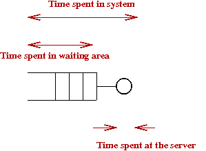
8.2 The single server queue
To learn how to write a next-event simulation, let's simplify the
queue example to a single server queue:
- This is the customary symbol:
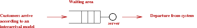
- Customers arrive to the queue (usually one-by-one) and queue
up for service.
- Upon receiving service, a customer leaves and does not return.
- The interarrivals are random, as are the service times for
each customer.
- All the interarrivals come from the same distribution.
- All the service times come from the same distribution.
- If the server is not occupied when a customer arrives,
there is no waiting
\(\Rightarrow\) service commences immediately.
- We are usually interested in the following statistics:
- What is the average waiting time?
- What is the average system time?
- What is the average number of customers in the waiting area?
- What is the average number of customers in the system?
Exercise 2:
Download and execute Queue.java,
which is a simulation of a single server queue.
Cursorily examine the code.
- What data structures are being used?
- Where in the code are interarrival times being generated? From what distribution?
- Where are service times being generated? From what distribution?
Let's now understand the details using an example:
- First consider interarrivals:
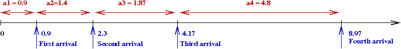
- Let rv \(A_i\) denote the \(i\)-th interarrival.
- Since all the \(A_i\)'s have the same
distribution \(\expt{A_i} = \expt{A_j}\) for
any \(i\) and \(j\).
\(\Rightarrow\) We'll use \(\expt{A}\) for the mean interarrival time.
- Suppose our random interarrival generator happens to
produce the particular values \(0.9, 1.4, 1.87, 4.8\) as
the first four interarrivals.
- Let \(a_1=0.9, a_2=1.4, a_3=1.87, a_4=4.8\).
\(\Rightarrow\) Here, \(a_i\) = the actual value produced
by the generator for the \(i\)-th interarrival.
Exercise 3:
Add code in method randomInterarrivalTime()
in Queue.java
to estimate the average interarrival time.
What does this number have to do with the value of
variable arrivalRate in the program?
- Next, consider the (random) service time needed by these
customers:
- Let rv \(S_i\) represent the service time needed
by the \(i\)-th customer
\(\Rightarrow\) \(S_i\) = \(i\)-th service time.
- As with the mean interarrival time, we'll let
\(\expt{S}\) denote the mean service time.
- As an example, the random generator for service times could
produce: \(2.3, 2.11, 1.68, 1.3\) as the first four
service times.
- Let \(s_1=2.3, s_2=2.11,
s_3=1.68, s_4=1.3\).
\(\Rightarrow\) Here, \(s_i\) = the actual value produced
by the generator for the \(i\)-th service time.
Exercise 4:
Add code in method randomServiceTime()
in Queue.java
to estimate the average service time.
- Now let us plot the departures along the time-line:
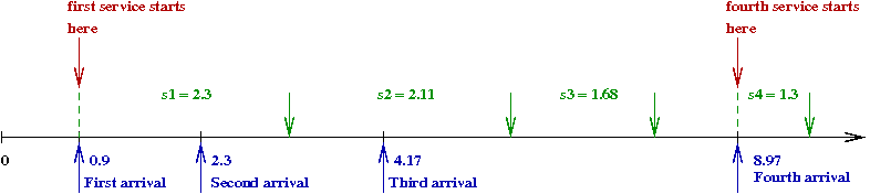
- First, notice that customer 1's service begins at 0.9
\(\Rightarrow\) It can't start earlier because customer 1 hasn't arrived yet!
- Thus, the first departure occurs at \(t = 0.9 + 2.3 = 3.2\).
- Since customer 2 arrives before customer 1 finishes, customer 2's
service begins at \(t = 3.2\) and ends at \(t = 3.2 + 2.11 = 5.31\).
- Note: since customer 3 finishes before customer 4 arrives,
we start customer 4's service at \(t = 8.97\).
\(\Rightarrow\) Customer 4 departs at \(t = 8.97 + 1.3 = 10.27\).
- We'll now plot the number in the system against time:
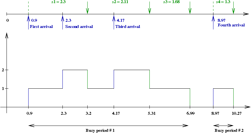
- The number increases by one at each arrival, and decreases
by one at each departure.
- A contiguous block when the server is busy is called a
busy period.
Exercise 5:
Suppose five customers arrived with interarrivals
\(a_1=1.0, a_2=2.0, a_3=1.0, a_4=1.5, a_5=3.5\)
with service times
\(s_1=1.1, s_2=3.5, s_3=1.5, s_4=2.5, s_5=2.0\).
For this data, draw the above graph that plots
the number in the system against time.
- If we were to advance the clock in fixed, small steps, it
might look like this:
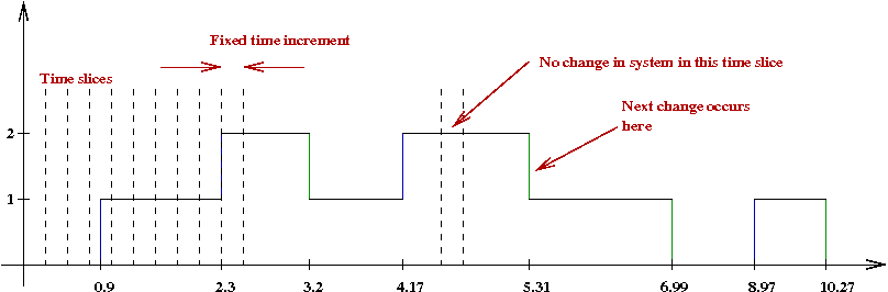
- The smaller the increment, the more the computation.
- Notice that no change occurs in most time slices.
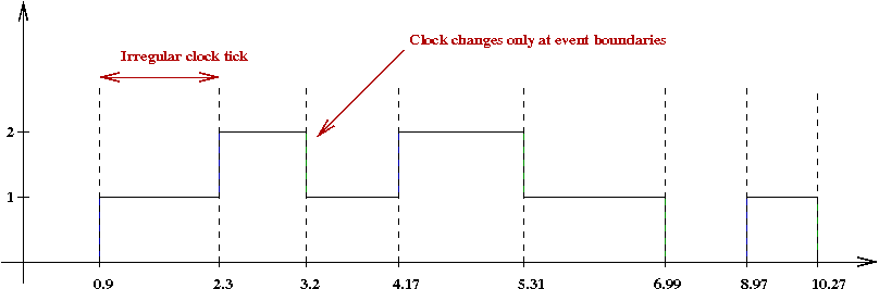
- In a next-event simulation, we will advance the clock
only at event occurence times:
There are two key ideas in next-event simulation. Let's explore these
using our queue example:
- The first idea: because the clock advances from event to event,
the main loop of a simulation involves event-processing:
     while not over
         event = getNextEvent ()        // Get the next event (from some data structure).
         clock = event.time             // Advance the clock to the next event's time of occurence.
         handleEventDetails (event)     // Update simulation variables of interest.
     endwhile
- In more detail, the first idea would look like this:
     // Generate all the arrival times
     for i=1 to numArrivals
         ai = randomInterrival ()
         arrivalList.add (ai)
     endfor

     // Generate all the service times
     for i=1 to numArrivals
         si = randomServiceTime ()
         serviceTimeList.add (si)
     endfor

     // Now simulate.
     while not over
         event = getNextEvent ()        // This method will use arrivalList and serviceList.
         clock = event.time
         handleEventDetails (event)
     endwhile
For large simulations (millions of events), this incurs a
large storage cost.
- The second (better) idea: we do not need to have all events generated
ahead of time.
- Observe that we don't need to generate events until
they're needed.
\(\Rightarrow\) We'll generate as we go.
- Thus, in pseudocode:
     while not over
         event = getNextEvent ()
         clock = event.time
         if event.type = arrival
             handleArrival (event)
             generateNextArrival ()      // Here's where the next ai is generated.
         else
             handleDeparture (event)
             generateNextDeparture ()    // Generate the next si.
         endif
     endwhile
Where are events stored?
- We will need a data structure to store events
\(\Rightarrow\) For now, we will call this the event-list.
- Thus the method call
event = getNextEvent ()
should return the next event from this list.
- But which event?
\(\Rightarrow\) The event with the earliest time.
- A data structure that maintains order and returns the least
value is called a priority queue.
- Thus, Java code for a queue simulation might look like this:
public class Queue {

    // List of forthcoming events.
    PriorityQueue<Event> eventList;

    // The system clock, which we'll advance from event to event.
    double clock;

    void simulate (int maxCustomers)
    {
        init ();                                     // Initialize stats variables.

        // Simulate for a given max # of customers.
        while (numCustomers < maxCustomers) {
            Event e = eventList.poll ();             // Remove event with earliest time.
            clock = e.eventTime;                     // Advance the clock.
            if (e.type == Event.ARRIVAL) {           // Handle the event details.
                handleArrival (e);
            }
            else {
                handleDeparture (e);
            }
        }

        stats ();                                    // Print stats like "avg wait time"
    }
}
Exercise 6:
Examine method simulate()
in Queue.java
and verify that it has this structure.
Then examine init() to see if the initialization
makes sense. Why is there a call to scheduleArrival()
in init()?
Event handling details:
- First, let's ask what we need to do when an arrival occurs:
- If the waiting area already has customers
\(\Rightarrow\) Add new customer to waiting area.
- If, instead, the server is available
\(\Rightarrow\) Schedule the completion of service (departure).
- In either case, schedule the next arrival
\(\Rightarrow\) Create a random interarrival, add the clock and put
that arrival into the event list.
- Thus, our Java code would look like:
    void handleArrival (Event e)
    {
	numCustomers ++;
	if ( ... ) {  // This is the only customer => schedule a departure.
            // Create a random service time, put the event on the event list.
	    scheduleDeparture ();
	}
        // Schedule the next arrival: create a random arrival time etc.
	scheduleArrival ();
    }
- What happens with a service completion?
- If there aren't any more customers
\(\Rightarrow\) Nothing to be done.
- If there are more customers waiting
\(\Rightarrow\) Schedule the service of the one waiting longest.
- Thus, in Java
    void handleDeparture (Event e)
    {
	numDepartures ++;
        if ( ... )  { // If there are more waiting customers
            // Create a random service time, put the event on the eventlist.
	    scheduleDeparture ();
        }
    }
The other important data structure:
- Consider how we estimate a customer's system time:
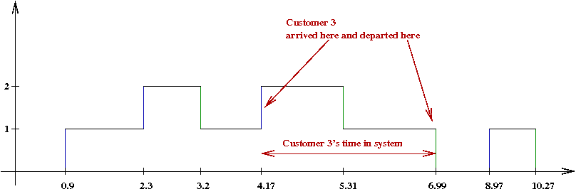
- When customer 3 leaves, we need to know the arrival time
for that customer
\(\Rightarrow\) Need to store this somewhere.
- Then compute
Customer 3's time in system = departureTime - arrivalTime
- But where do we store each customer's arrival time?
- One option: a simple list that stores the arrival time for
each customer.
- Note: once a customer departs, we don't need the arrival
time anymore.
\(\Rightarrow\) Can remove that customer from data structure.
\(\Rightarrow\) Only currently waiting or serviced customers in data structure.
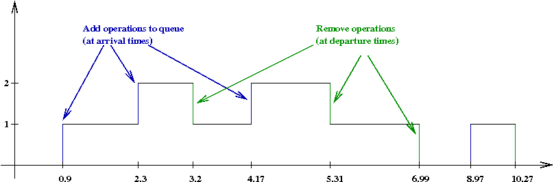
- Notice the operations: add and remove
- Add operation: when a newly arriving customer is processed.
- Remove operation: when departing customer is processed.
- Thus, what we need is a queue (the data structure,
that is).
- At arrival time,
    void handleArrival (Event e)
    {
	numCustomers ++;
        Customer c = new Customer ();
	queue.add (c);                      // Add the new customer.
	if (queue.size() == 1) {            // Is this the only customer in the system?
	    scheduleDeparture ();           // Schedule this "only" person's service completion.
	}
	scheduleArrival ();
    }
- When handling a departure ...
    void handleDeparture (Event e)
    {
	numDepartures ++;
	Customer c = queue.removeFirst ();

        // This is the time from start to finish for this customer:
        double timeInSystem = clock - c.arrivalTime;

        // Maintain total (for average, to be computed later).
	totalSystemTime += timeInSystem;

	if (queue.size() > 0) {           // Is there a waiting customer?
	    scheduleDeparture ();         // If so, schedule a departure.
	}
    }
We're now in a position to examine a complete simulation:
- First, in pseudocode
     Algorithm: simulate (M)
     Input: M - maximum number of arrivals
     1.   initialize stats, queue, eventList;
     2.   while numArrivals < M
     3.       event = getNextEvent ()
     4.       clock = event.time
     5.       if event.type = arrival
     6.           handleArrival (event)
     7.       else
     8.           handleDeparture (event)
     9.       endif
     10.  endwhile
     11.  print stats


     Method: handleArrival (e)
     Input:  event e
     1.  numArrivals = numArrivals + 1
     2.  c.arrivalTime = clock
     3.  queue.add (c)
     4.  if queue.size = 1
     5.      scheduleDeparture ()
     6.  endif
     7.  scheduleArrival ()


     Method: handleDeparture (e)
     Input:  event e
     1.  c = queue.remove ()
     2.  updateStats (clock - c.arrivalTime)
     2.  if queue.size > 0
     3.      scheduleDeparture ()
     4.  endif
- The Java version is not very different:
(source file)
public class Queue {

    // A data structure to store customers.
    LinkedList<Customer> queue;

    // A data structure for simulation: list of forthcoming events.
    PriorityQueue<Event> eventList;

    // The system clock, which we'll advance from event to event.
    double clock;

    void init ()
    {
        queue = new LinkedList<Customer> ();
        eventList = new PriorityQueue<Event> ();
        clock = 0.0;
        // Important: we need to start by scheduling the first arrival.
        scheduleArrival ();
    }

    void simulate (int maxCustomers)
    {
        init ();

        while (numArrivals < maxCustomers) {
            Event e = eventList.poll ();
            clock = e.eventTime;
            if (e.type == Event.ARRIVAL) {
                handleArrival (e);
            }
            else {
                handleDeparture (e);
            }
        }

        stats ();
    }


    void handleArrival (Event e)
    {
	numArrivals ++;
	queue.add (new Customer (clock));
	if (queue.size() == 1) {
	    // This is the only customer => schedule a departure.
	    scheduleDeparture ();
	}
	scheduleArrival ();
    }


    void handleDeparture (Event e)
    {
	numDepartures ++;
	Customer c = queue.removeFirst ();

        // This is the time from start to finish for this customer:
        double timeInSystem = clock - c.arrivalTime;

        // Maintain total (for average, to be computed later).
	totalSystemTime += timeInSystem;

	if (queue.size() > 0) {
	    // There's a waiting customer => schedule departure.
	    scheduleDeparture ();
	}
    }

}
- The code for each event and customer is simple:
class Customer {
    double arrivalTime;
    public Customer (double arrivalTime)
    {
        this.arrivalTime = arrivalTime;
    }
}


class Event implements Comparable {

    public static int ARRIVAL = 1;
    public static int DEPARTURE = 2;
    int type = -1;                     // Arrival or departure.
    double eventTime;                  // When it occurs.

    public Event (double eventTime, int type)
    {
	this.eventTime = eventTime;
	this.type = type;
    }

    public int compareTo (Object obj)         // This is needed to make events Comparable.
    {
        Event e = (Event) obj;
        if (eventTime < e.eventTime) {
            return -1;
        }
        else if (eventTime > e.eventTime) {
            return 1;
        }
        else {
            return 0;
        }
    }

}
What do we want to get out of the simulation?
- First, let's examine the time-in-system:
- This is the time from arrival to departure (including service).
- Let rv \(D_i\) represent customer \(i\)'s
time spent in the system.
- We want to estimate
$$
\frac{1}{n} \sum_i D_i
$$
- Notice where we accumulate such values in method handleDeparture:
    void handleDeparture (Event e)
    {
	numDepartures ++;
	Customer c = queue.removeFirst ();

        // This is the time from start to finish for this customer:
        double timeInSystem = clock - c.arrivalTime;

        // Maintain total (for average, to be computed later).
	totalSystemTime += timeInSystem;

        // ...
    }
- Then, later we estimate
    void stats ()
    {
        // ...

	avgSystemTime = totalSystemTime / numDepartures;
    }
Exercise 7:
Execute Queue.java
to estimate the average time in system.
- Next, consider the time spent in the waiting area:
- Let rv \(W_i\) represent customer \(i\)'s
waiting time (waiting for service).
- Notice that some customer's don't wait at all.
- We want to estimate
$$
\frac{1}{n} \sum_i W_i
$$
- Extracting waiting times needs a little thought:
\(\Rightarrow\) We need to do this just before a customer enters service.
- Notice where in the code this occurs:
    void handleDeparture (Event e)
    {
        // ...

	if (queue.size() > 0) {

            // We can't yet remove this customer
            // but we need to access this customer to extract the arrival time.
	    Customer waitingCust = queue.get (0);

            // This is the time spent only in waiting:
            double waitTime = clock - waitingCust.arrivalTime;

            // Accumulate total.
            totalWaitTime += waitTime;

            // ...
	}
    }
Exercise 8:
Execute Queue.java
to estimate the average waiting time. Subtract this
from the estimate of the average system-time.
What do you get? Is it what you expect?
8.3 The single server queue - some analysis
The idea of a rate:
Exercise 11:
Fix the service rate at \(\mu=1\) and vary
the arrival rate: try \(\lambda = 0.5, 0.75, 1.25\).
What do you observe when \(\lambda = 1.25\)?
Relationship between \(\lambda\) and \(\mu\):
- First consider the case \(\lambda \geq \mu\):
\(\Rightarrow\) This is the same as saying \(\expt{A} \lt \expt{S}\).
\(\Rightarrow\) There are more arrivals than the server can handle (on average).
\(\Rightarrow\) The number in the waiting area gradually increases
\(\Rightarrow\) Grows without bound (blows up).
- Suppose we fix \(\mu=1\) and vary \(\lambda\)
between \(0\) and \(1\).
- Next, recall that
\(D_i\) = customer \(i\)'s time spent in the system.
- Let \(d\) denote the mean system time.
$$
\frac{1}{n} \sum_i D_i \; \to \; d
$$
- Clearly, \(d\) depends on both \(\mu=1\) and \(\lambda\).
We'll use the notation \(d(\lambda,\mu)\) to show
that \(d\) is a function of both.
- We've established one fact already
As \(\lambda \to \mu\),
we get \(d \to \infty \).
- What about the other end, when \(\lambda \to 0\)?
Exercise 12:
What about it?
- Next, let's systematically consider different values of
\(\lambda\).
Exercise 13:
Vary \(\lambda\) as follows: \(0.1, 0.2, ..., 0.9\)
and estimate \(d\).
What is the shape of the function
\(d(\lambda,\mu)\)?
Next, let's focus on the number of customers in the system:
- An arriving customer either gets service immediately or has to wait.
\(\Rightarrow\) An arriving customer either sees zero customers in the
system or some non-zero number of customers.
- Let \(M_i\) be the number of customers
seen by customer \(i\) at the moment of arrival.
- We want to estimate
$$
\frac{1}{n} \sum_i M_i
$$
- Let \(m\) denote the mean number in the system (as seen
by an arriving customer), i.e.,
$$
\frac{1}{n} \sum_i M_i \; \to \; m
$$
Exercise 14:
For \(\lambda=0.75\) and \(\mu=1\), estimate \(m\).
Then compute \(\frac{m}{d}\), where \(d\) is the mean system time.
Little's Law:
- Consider the three numbers \(d, m\) and \(\lambda\).
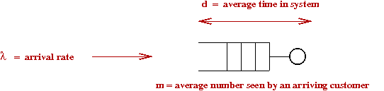
- Now consider an "average" customer.
- How much time does Mr.Average spend in the system?
\(\Rightarrow\) \(d\).
- During this period \(d\), how many arrivals occur (on average)?
\(\Rightarrow\) \(\lambda d\).
- When Mr.Average departs, what is the average number of
customers remaining in the system?
\(\Rightarrow\) \(m\).
- But these remaining customers are the ones who came
during Mr.Average's sojourn
\(\Rightarrow\) \(m = \lambda d\) (on average).
\(\Rightarrow\) This is called Little's Law.
- Little's Law can be shown to hold in great generality.
\(\Rightarrow\) Doesn't have to do with queueing systems.
Other measures of interest:
- We have thus far measured the average (number in the system,
system time).
- Often, we are also interested in particular probabilities
e.g., the system utilization = \(\probm{server is busy}\).
- In an underutilized system, the server is unused.
\(\Rightarrow\) This might suggest allowing an increased arrival rate.
- Sometimes, it's useful to know the distribution
instead of the mean.
Exercise 15:
For \(\lambda=0.75\) and \(\mu=1\),
estimate the probability that an arriving customer finds
the server free. Try this for \(\lambda = 0.5, 0.6\) as well.
Can you relate this probability to \(\lambda=0.75\) and \(\mu=1\)?
Exercise 16:
We will focus on two distributions: the distribution of
the number in the system, and the system time.
Let rv \(M\) denote the number of customers seen by
an arriving customer, and let rv \(D\) denote the system
time experienced by a random customer.
- Is \(M\) discrete or continuous? What about \(D\)?
What is the range of \(M\)? Of \(D\)?
- For \(\lambda=0.75\) and \(\mu=1\),
obtain the appropriate histogram of \(M\).
Which well-known distribution does this look like?
- For \(\lambda=0.75\) and \(\mu=1\),
obtain the appropriate histogram of \(D\).
Which well-known distribution does this look like?
Note: use
PropHistogram.java
or
DensityHistogram.java
as appropriate.
8.4 An example with multiple queues
Consider this example with three queues:
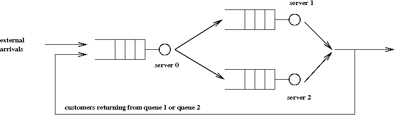
- There are three servers: 0, 1, 2.
- Each server has a waiting area
\(\Rightarrow\) We'll call the combination of server and waiting area: a queue.
\(\Rightarrow\) There are three queues.
- Customers arrive from the outside and enter queue 0.
\(\Rightarrow\) We'll use exponentially-distributed interarrival times.
- A customer departing from queue 0 goes to either queue 1 or
queue 2 (to receive service from server 1 or 2).
\(\Rightarrow\) We'll use a simple choice-model: a customer chooses
between 1 and 2 with equal probability.
- Upon departing either queue 1 or 2, a customer may either
leave the system or may return for another sojourn through the system.
\(\Rightarrow\) Some fraction \(q\) of customers return.
- Our goal: to understand how to write a next-event simulation
of this system.
Before writing the simulation, let's look at possible applications:
- A web server farm:
- HTTP requests come from browsers (users) to a website.
- The website has a front-end server that then routes
the request to one of two back-end servers.
- The backend servers perform the computation required and
send the results back to the client browser.
- To improve response times, the requests are divided between
the two backend servers.
- Some requests result in an immediate follow up (this is the
feedback part).
- A dual-core processor:
- The first queue represents the operating system overhead in
scheduling.
- The other two queues are the two processors.
- Some jobs return after receiving a slice of CPU time.
- Machine-shop:
- A factory makes a product that need two types of machining.
- There are three machines used: machine 0 does the first
type, and machines 1 or 2 do the second type.
- Some products need finishing touches or re-working, and go
back after inspection.
- Evil bureaucracy:
- You need two kinds of approval on your application.
- Desk 0 does the first kind, and desks 1,2 do the second kind.
- Because they are nit-picky, you might have to go back
through the system.
Applications of queueing systems in general:
- Queueing systems are used in a variety of situations:
computer systems, manufacturing, service-centers.
- These systems share the following characteristics:
- There are multiple "points of service" or stages of service.
- Customers (jobs, tasks) are routed amongst these servers.
- Each server has a waiting area.
- Service times are often random (with some mean).
OK, back to our example:
- First, let's identify the parameters:
- The external arrival rate.
- The mean service time at each server
\(\Rightarrow\) Alternatively, the service rate for each server.
- The fraction of customers who return.
Thus, our code will have something like
public class ThreeQueue {

    // Fraction that return to start.
    double fracReturn = 0.1;

    // Avg time between arrivals = 1.0, avg time at server=1/0.75.
    double arrivalRate = 1.0;
    double[] serviceRates = {2.0, 1.0, 1.0};

}
- Next, let's look at the data structures needed:
- We'll use one queue (list) data structure for each queue.
- And we'll use a single event list for the whole simulation.
public class ThreeQueue {

    // Fraction that return to start.
    double fracReturn = 0.1;

    // Avg time between arrivals = 1.0, avg time at server=1/0.75.
    double arrivalRate = 1.0;
    double[] serviceRates = {2.0, 1.0, 1.0};

    // Three queues: queue[0], queue[1], queue[2]
    LinkedList<Customer>[] queues;

    PriorityQueue<Event> eventList;

}
- The main simulation loop will be exactly the same:
    void simulate (int maxCustomers)
    {
        init ();

        while (numDepartures < maxCustomers) {
            Event e = eventList.poll ();
            clock = e.eventTime;
            if (e.type == Event.ARRIVAL) {
                handleArrival (e);
            }
            else {
                handleDeparture (e);
            }
        }

        stats ();
    }
Note: the structure of the simulation is the same.
\(\Rightarrow\) It's only the event-handling details that differ.
- To handle an external arrival:
    void handleArrival (Event e)
    {
	numArrivals ++;
	queues[0].add (new Customer (clock));      // Place external arrival in queue[0]
	if (queues[0].size() == 1) {
	    scheduleDeparture (0);                 // Schedule departure if needed.
	}
	scheduleArrival ();
    }
Notice that scheduleDeparture() now takes a parameter -
the queue number.
- Thus, in scheduleDeparture():
    void scheduleDeparture (int i)
    {
	double nextDepartureTime = clock + randomServiceTime (i);
	eventList.add (new Event (nextDepartureTime, Event.DEPARTURE, i));
    }

    double randomServiceTime (int i)
    {
        // Each server may have a different rate \(\Rightarrow\) different exponential parameters.
	return exponential (serviceRates[i]);
    }
- How is a departure event handled? In pseudocode
      Method: handleDeparture (k)
      Input: k, the queue from which the departure occurs
      1.   if k = 0
      2.       send to queue 1 or queue 2
      3.   else
      4.       if uniform() < q
      5.           send back to queue 0
      6.       else
      7.           remove from system
      8.       endif
      9.   endif
Exercise 17:
Download and execute the above simulation:
ThreeQueue.java
- What is the average system time?
- Examine the code to see where the system time is being accumulated.
- Change the queue choice (between 1 and 2) to
"shortest-queue" instead of "uniform-random" and see the
difference this makes.
- In what kind of application is "uniform-random" better
than "shortest-queue"?
- Measure the rate of departures from the system and explain
the value you get.
8.5 Synchronous simulations
What is a synchronous simulation?
- Recall that in a next-event simulation, the clock jumps
by random amounts
\(\Rightarrow\) From one event occurence to the next.
- We could, loosely, call this an asychronous simulation.
- In contrast, in a synchronous simulation, the clock
steps are the integers.
\(\Rightarrow\) Time proceeds in fixed steps.
- Furthermore, it's usually the case that the actual time
in a step doesn't matter
\(\Rightarrow\) The steps are all that's needed.
Exercise 18:
Download and execute
Boids.java.
About the boids simulation:
- It is meant to simulate the flocking behavior of birds.
- Each bird, except the "leader," looks at other birds and tries to fly towards
them.
- The leader picks a random direction in which to fly.
- To make it interesting, we occasionally change the leader.
- We will use a synchronous simulation:
     Algorithm: boidsSimulation (n)
     Input: N - the number of steps to simulate
     1.   boids = random initial locations
     2.   for n=1 to N
     3.       nextStep ()               // This is one step in N steps.
     4.   endfor


     Method: nextStep ()
     1.   newBoidLocations = applyBoidRules ()      // Move according to boid rules.
     2.   for i=1 to numBoids
     3.       boids[i] = newBoidLocations[i]        // Set new locations in one shot.
     4.   endfor
- In the Boids.java program:
    void simulate ()
    {
        init ();
        for (int n=0; n<numSteps; n++) {
            nextStep ();
            try {                               // Sleep for animation effect.
                Thread.sleep (100);
            }
            catch (InterruptedException e) {
                break;
            }
            repaint ();
        }
    }


    void nextStep ()
    {
        // The new locations will be stored here temporarily.
	Point[] newLocations = new Point [numBoids];

	// Is it time to change the leader?
	if (RandTool.uniform() < leaderChangeProb) {
	    leader = RandTool.uniform (0, numBoids-1);
	    leaderTheta = RandTool.uniform (0.0, Math.PI);
	}

        // Except for the leader, move the others towards neighbors.
	for (int i=0; i<numBoids; i++) {
	    if (i == leader) {
                // Apply different rules for leader.
                newLocations[leader] = moveLeader ();
	    }
            else {
                newLocations[i] = moveOther (i);
            }
        }

        // Synchronous update for all.
        for (int i=0; i<numBoids; i++) {
            boids[i] = newLocations[i];
        }
    }
Let's see what an asynchronous version of boids might look like:
- In the asynchronous version:
- Each boid moves independently.
- Each moves and then sleeps for a random amount of time.
\(\Rightarrow\) The sleep time will be exponentially distributed.
- Our main simulation loop will look like:
    void simulate ()
    {
        init ();

        for (int n=0; n<numSteps; n++) {

            // Next-event simulation:
            Event event = eventList.poll ();
            nextStep (event.i);
            scheduleNextMove (event.i);

            // Sleep for animation effect ... etc
        }
    }
Thus, the next boid to "wake up" is moved, and its next wake-up
time is scheduled.
- In nextStep() we now only focus on moving the one
boid that's awake:
    void nextStep (int i)
    {
	// Is it time to change the leader?
	if (RandTool.uniform() < leaderChangeProb) {
	    leader = RandTool.uniform (0, numBoids-1);
	    leaderTheta = RandTool.uniform (0.0, Math.PI);
	}

        // Except for the leader, move the others towards neighbors.
        if (i == leader) {
            // Apply different rules for leader.
            boids[i] = moveLeader ();
        }
        else {
            boids[i] = moveOther (i);
        }

        // Note: No need for copying over new locations.
    }
Exercise 19:
Download and execute
AsynchBoids.java.
What do you notice? Does it work?
Exercise 20:
Examine the code in the molecular simulation from
Module 4.
Is this synchronous or asynchronous?
Exercise 21:
Find a simulation of the Game-of-Life.
Is this synchronous or asynchronous?
Both synchronous and asynchronous simulations share some features:
- In the examples we've seen, there are fundamental units or
"particles" that are processed
- In queues, the particles are customers.
- In the boids example, the particles are boids.
- In molecular simulations, particles are molecules.
- Each particle is subject to "something random"
- Customers have random interarrivals, random service times,
and random routing.
- Boids have random movements (especially the leader).
- Molecules have random movements.
- The particles are also subjected to non-random rules:
- Customers wait in order of arrival, they are served one at
a time.
- Boids (other than the leader) move according to others.
- Molecular movement occurs in short distances. Collisions
result in reactions.
Agent simulations:
- Agent simulations are usually intended to model some
higher-level entities such as:
- People in an economy:
The interactions are trades or buy-sell transactions.
- Animals in a competitive environment
\(\Rightarrow\) e.g., predator-prey.
- Computationally, an agent simulation is no different
than a particle simulation.
- Most agent simulations have some spatial aspect
\(\Rightarrow\) e.g., a 2D "landscape"
- Predator-prey example:
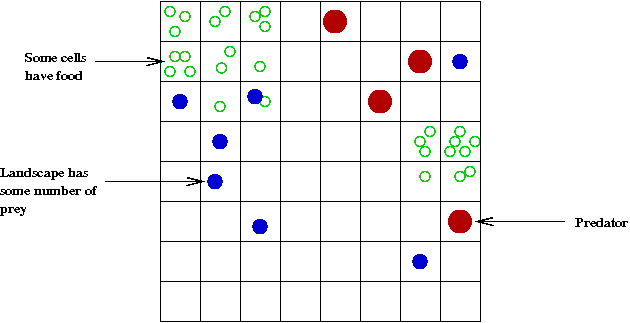
- The landscape: \(M \times M\) cells.
- Two types of creatures: prey and predator.
- At time-step \(t\), let
\(N_1(t)\) = number of prey
\(N_2(t)\) = number of predators.
- Some cells have food (needed by prey).
- Example of rules for predator-prey simulation:
- Movement rules: e.g., each animal moves to a random
neighboring cell.
- If the cell has food, a prey animal consumes food.
\(\Rightarrow\) Else, prey dies off.
- If a predator is in the same cell as a prey, prey is consumed
\(\Rightarrow\) predator survives.
- Examples of simulation objectives:
- Study correlation with food availability, speed of movement.
- What happens to \(N_1(t)\) and \(N_2(t)\)
as \(t\) gets large?
- Is there a stable population or is there natural
fluctuation as in the ODE model?
- What is the effect of death rates amongst predators? A
sudden catastrophe?
- Multiple predators, multiple prey.
8.6 A simple one-particle simulation
The raindrop problem:
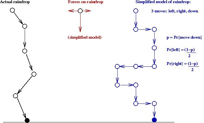
- Our single particle will be a raindrop.
\(\Rightarrow\) We'll model a raindrop falling down, buffeted by winds.
- Our model will be simple:
- A raindrop is a point particle.
- It can move down, left or right.
\(\Rightarrow\) A down-move occurs with probability \(p\), and a
left move occurs with probability \(\frac{(1-p)}{2}\).
- The distance moved is a fixed constant, \(s\).
- The raindrop is dropped from a height \(h\).
- When the raindrop hits the ground, we stop.
- What do we want to do with a simulation?
- Measure the distribution of where the rain drop falls.
- Measure the distribution of the time taken.
- The two rv's of interest are:
- Let rv \(X\) = the point (along the x-axis) where the
raindrop hits the ground.
\(\Rightarrow\) We'll assume the drop point is along the y-axis.
- Let rv \(T\) denote the time taken.
- The simulation (for a single trial) is quite simple
     Algorithm: raindrop (h, s, p)
     Input: h - starting height, s = stepsize, p = Pr[move down]
     1.   x = 0
     3.   t = 0
     4.   while h > 0
     5.      if uniform() < p
     6.          h = h - s                        // Move down
     7.      else if uniform() < 0.5
     8.          x = x + s                        // Move right
     9.      else
     10          x = x - s                        // Move left
     11      endif
     12      t = t + 1
     13   endwhile
     14.  return x, t
Exercise 22:
Fill in code in Raindrop.java
to obtain histograms of \(X\) and \(T\) respectively.
Use \(s=1, h=10, p=0.5\).
- What is the likely distribution of \(X\)?
- Vary \(h\): try \(h = 20, 30, 40, 50\). What is the
relationship between \(\expt{T}\) and \(h\)?
Note: use
PropHistogram.java
or
DensityHistogram.java
as appropriate.
Exercise 23:
Do you know the historical significance of the distributions
of \(X\) and \(T\)?
8.7 The eventlist data structure
A data structure for an eventlist must support two operations:
- insert: insert a new element into the collection.
- extractMin: remove the smallest element in the collection.
- The implicit assumption: elements can be ordered from
"smallest" to "largest".
\(\Rightarrow\) Usually based on some numeric value.
- In a next-event simulation:
- The elements are events.
- The order is based on the time of occurence of an event.
- In the CS jargon, such a data structure is called a
priority queue.
\(\Rightarrow\) The value used in ordering is called an element's priority.
- In a simulation:
priority = event's time.
\(\Rightarrow\) Here, extractMin will remove the smallest-priority element.
Exercise 24:
What is the size of the eventlist for the single-server queue?
For the three-queue example?
When is this data structure important?
- When the eventlist becomes large.
- The eventlist becomes large in some applications:
\(\Rightarrow\) e.g., an asynchronous simulation with thousands (or
millions) or particles.
- Suppose we use a sorted linked-list:
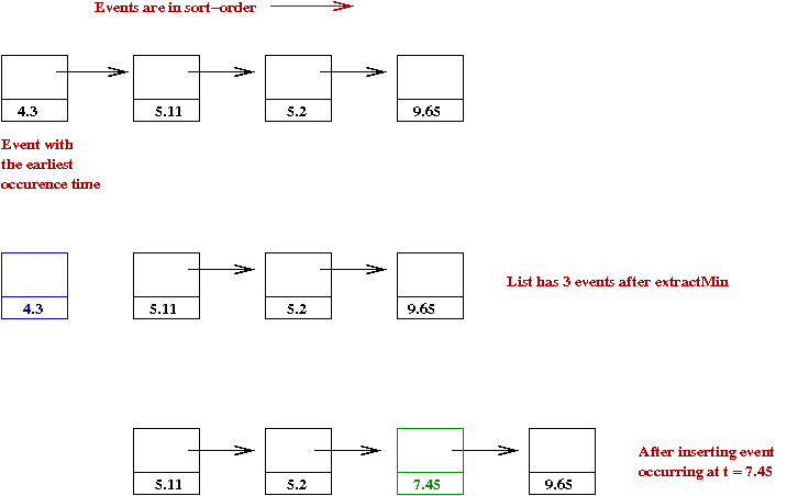
- For extractMin, remove and return the first element.
- For insert, insert a new event in correct position
in list.
Exercise 25:
If the eventlist has \(n\) events, how long does it
take for each operation (in order-notation)?
Exercise 26:
If instead of a sorted-list, we use an unsorted list,
how long does each operation take?
Better data structures:
- Using a binary heap, each operation can be done
in \(O(\log n)\) time.
- For an explanation of how a binary heap works,
see Module 2 of the
Algorithms course.
- Alternatives to the binary heap include: Binomial heap,
Fibonacci heap and the run-relaxed heap.
8.8 Summary
There are several types of simulation:
- Continuous-system simulation:
- These are essentially differential equations.
\(\Rightarrow\) Usually a system of equations (ODEs).
- Fixed, small time steps, \(\Delta t\).
- No randomness.
- Typical goal: to compute the time-evolution of continuous functions.
- Example:
\(v'(t) = a\)
\(d'(t) = v\)
Goal: compute \(d(t)\) (distance as a function of time).
- Next-event simulation:
- Key entities (particles) are discrete.
- Particles are subjected to randomness in some form.
- Events occur at random times.
\(\Rightarrow\) Nothing of significance happens between events.
- Clock is advanced from event to event.
- Synchronous simulation:
- Time proceeds in fixed steps
\(\Rightarrow\) The steps are numbered 1, 2, 3,..., and size usually has no meaning.
- The entire next state is computed for each particle (in
temporary variables).
\(\Rightarrow\) Switch to next state all at once.
The world of simulation:
- Sophisticated random generation techniques.
\(\Rightarrow\) Techniques for efficient, statistically-sound generation.
- Statistical techniques for simulation:
e.g., rare-event simulation, variance reduction.
- Simulation of large systems:
\(\Rightarrow\) Parallel or distributed simulation, simulation approximation.
- Continuous-system simulation:
\(\Rightarrow\) Specialized algorithms for different types of differential equations.
- Agent-based simulation (like Boids):
\(\Rightarrow\) Large application area (economics, sociology).
- Simulation optimization
\(\Rightarrow\) How to optimize parameters in a simulation.
- Simulated (virtual) worlds
\(\Rightarrow\) 3D graphics, modeling worlds, realistic physics simulation.
- Specialized applications:
\(\Rightarrow\) e.g., queueing simulations, molecular simulations, complex systems.
© 2008, Rahul Simha