\(
\newcommand{\blah}{blah-blah-blah}
\newcommand{\eqb}[1]{\begin{eqnarray*}#1\end{eqnarray*}}
\newcommand{\eqbn}[1]{\begin{eqnarray}#1\end{eqnarray}}
\newcommand{\bb}[1]{\mathbf{#1}}
\newcommand{\mat}[1]{\begin{bmatrix}#1\end{bmatrix}}
\newcommand{\nchoose}[2]{\left(\begin{array}{c} #1 \\ #2 \end{array}\right)}
\newcommand{\defn}{\stackrel{\vartriangle}{=}}
\newcommand{\rvectwo}[2]{\left(\begin{array}{c} #1 \\ #2 \end{array}\right)}
\newcommand{\rvecthree}[3]{\left(\begin{array}{r} #1 \\ #2\\ #3\end{array}\right)}
\newcommand{\rvecdots}[3]{\left(\begin{array}{r} #1 \\ #2\\ \vdots\\ #3\end{array}\right)}
\newcommand{\vectwo}[2]{\left[\begin{array}{r} #1\\#2\end{array}\right]}
\newcommand{\vecthree}[3]{\left[\begin{array}{r} #1 \\ #2\\ #3\end{array}\right]}
\newcommand{\vecdots}[3]{\left[\begin{array}{r} #1 \\ #2\\ \vdots\\ #3\end{array}\right]}
\newcommand{\eql}{\;\; = \;\;}
\newcommand{\eqt}{& \;\; = \;\;&}
\newcommand{\dv}[2]{\frac{#1}{#2}}
\newcommand{\half}{\frac{1}{2}}
\newcommand{\mmod}{\!\!\! \mod}
\newcommand{\ops}[1]{\;\; #1 \;\;}
\newcommand{\implies}{\Rightarrow\;\;\;\;\;\;\;\;\;\;\;\;}
\newcommand{\prob}[1]{\mbox{Pr}\left[ #1 \right]}
\newcommand{\probm}[1]{\mbox{Pr}\left[ \mbox{#1} \right]}
\definecolor{dkblue}{RGB}{0,0,120}
\definecolor{dkred}{RGB}{120,0,0}
\definecolor{dkgreen}{RGB}{0,120,0}
\newcommand{\plss}{\;\; + \;\;}
\)
Module 6: Elementary Probability - Computing with Events
6.1 Overview
Probability can be somewhat difficult and counterintuitive.
\(\Rightarrow\) It's better to approach the subject in stages.
Stages of learning in probability:
- Elementary probability (This module):
- Learn how to reason about coin flips, die rolls and the like.
- Understand sample spaces, events and what
probability means.
- Learn about combining events, conditional probability,
total-probability, and Bayes' rule.
- Be able to solve simple word problems of this kind:
- A biased coin has probability 0.7 of showing heads when tossed.
What is the probability of obtaining exactly 4 heads in 8 tosses?
- I have two coins, one of which is fair (Pr[heads]=0.5)
and the other biased (Pr[heads]=0.7). I pick one of them
randomly and flip 8 times. If I obtain 4 heads (in 8 tosses)
what is the probability that I picked the fair coin?
- Core probability:
- The concepts of: random variable, distribution, expectation.
- A few well-known discrete and continuous distributions.
- Difference between CDF and PDF.
- Joint distributions, conditional distributions, independence.
- Laws of large numbers and Central Limit Theorem.
- Elementary stats: mean, variance, confidence intervals.
- Simulation:
- How to generate random values from given distributions.
- How to write a discrete-event simulation.
- Simulation data structures.
- (Assorted) Intermediate topics:
- Conditional distributions, Markov chains.
- Queueing Theory.
- Monte Carlo methods.
- Hidden-Markov models.
Discrete vs. continuous:
- The discrete-continuous dichotomy in probability manifests in two different ways.
- Actual probabilities are themselves real numbers
\(\Rightarrow\) That part is always continuous
- However, the outcomes of an experiment may be
- discrete: e.g., result of a coin flip
- continuous: e.g., location of a robot in the (x,y) plane
- It's usually easier to understand discrete probability,
so we'll start with that.
About this module:
- We will focus on elementary probability
\(\Rightarrow\) As usual, we will take a computational approach.
- But first, let's familiarize ourselves with some classic examples.
6.2 Coin flips
Let's begin with some simple coin flips:
- Consider the following program
(source file)
public class CoinExample {

    public static void main (String[] argv)
    {
        // Flip a coin 5 times.
        Coin coin = new Coin ();
        for (int i=0; i<5; i++) {
            int c = coin.flip ();                           // Returns 1 (heads) or 0 (tails).
            System.out.println ("Flip #" + i + ": " + c);
        }
    }

}
Exercise 1:
Download Coin.java,
CoinExample.java,
and RandTool.java.
Then compile and execute.
Exercise 2:
Download StrangeCoin.class.
This class models a biased coin in which Pr[heads] is not 0.5.
Write a program to estimate Pr[heads] for this coin.
Next, we'll estimate the probability that, if we flip a
biased (Pr[heads]=0.6)
coin twice, at least one flip resulted in heads:
(source file)
public class CoinExample2 {

    public static void main (String[] argv)
    {
        // "Large" # trials.
	double numTrials = 1000000;

        // Count # times desired outcome shows up.
	double numSuccesses = 0;

	Coin coin = new Coin (0.6);           // Pr[heads]=0.6

	for (int n=0; n<numTrials; n++) {
            // Notice what we're repeating for #trials: the two flips.
	    int c1 = coin.flip ();
	    int c2 = coin.flip ();

	    if ( (c1==1) || (c2==1) ) {
                // If either resulted in heads, that's a successful outcome.
		numSuccesses ++;
	    }
	}

        // Estimate.
	double prob = numSuccesses / numTrials;

	System.out.println ("Pr[At least 1 h in 2 flips]=" + prob + "  theory=" + 0.84);
    }

}
Note:
- Thus far, the appropriate number of trials to use seems arbitrary.
- To avoid casting, we declared both numTrials and
numSuccesses as double's.
Exercise 3:
Modify the above program, writing your code
in CoinExample3.java,
to estimate the probability of obtaining
exactly 2 heads in 3 flips. Can you reason about the theoretically
correct answer?
Exercise 4:
This exercise has to do with obtaining tails in the first two flips
using the biased (Pr[heads]=0.6):
- What is the probability that, in 3 flips, the third and only
the third flip results in heads?
- What is the probability that, with an unlimited number of
flips, you need at least three flips to see heads for the
first time?
- Why are these two probabilities different?
Modify the above example, writing your code
in CoinExample4.java
and
CoinExample5.java.
6.3 Dice
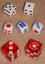
The following simple experiment rolls a die and estimates
the probability that the outcome is odd:
(source file)
public class DieRollExample {

    public static void main (String[] argv)
    {
	double numTrials = 1000000;
	double numSuccesses = 0;

	Die die = new Die ();

	for (int n=0; n<numTrials; n++) {

            // This is the experiment: a single roll.
	    int k = die.roll ();

            // This is what we're interested in observing:
	    if ( (k==1) || (k==3) || (k==5) ) {
		numSuccesses ++;
	    }
	}

	double prob = numSuccesses / numTrials;

	System.out.println ("Pr[odd]=" + prob + "  theory=" + 0.5);
    }

}
Exercise 5:
Roll a pair of dice (or roll one die twice).
What is the probability that the first outcome
is odd AND the second outcome is even?
Write code in DieRollExample2.java
to simulate this event. You will need
Die.java.
See if you can reason about this theoretically.
6.4 Cards
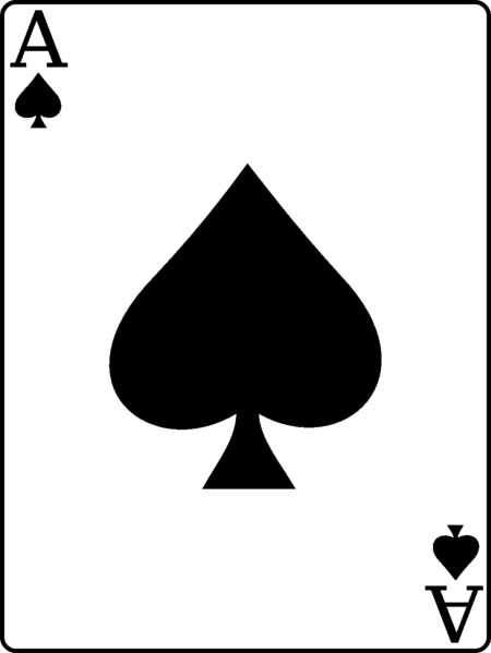
Let's now draw cards from a deck of cards:
- We'll number the cards 0,..,51.
- Convention: 0..12 (spades), 13..25 (hearts), 26..38
(diamonds), 39..51 (clubs)
- Type of drawing:
- We can draw with replacement
\(\Rightarrow\) Put the card back into the deck.
- Or, without replacement
\(\Rightarrow\) Draw further cards without putting back cards already drawn.
- We'll use the class CardDeck,
which has methods
int drawWithReplacement()
int drawWithoutReplacement()
isSpade (int c)
isHeart (int c)
isDiamond (int c)
isClub (int c)
Now consider this experiment:
- Draw a card without replacement, then draw a second card.
\(\Rightarrow\) What is the probability the second card is the Ace of Hearts?
- Here's a simple program to estimate this probability:
(source file)
public class CardExample {

    public static void main (String[] argv)
    {
	double numTrials = 100000;
	double numSuccesses = 0;

	for (int n=0; n<numTrials; n++) {
            // Note: we use a fresh pack each time because the cards aren't replaced.
	    CardDeck deck = new CardDeck ();
	    int c1 = deck.drawWithoutReplacement ();
	    int c2 = deck.drawWithoutReplacement ();
	    if (c2 == 13) {
		numSuccesses ++;
	    }
	}
	double prob = numSuccesses / numTrials;
	System.out.println ("Pr[c2=13]=" + prob + "  theory=" + (1.0/52.0));
    }

}
- We can test membership in a suit as follows:
    int c = deck.drawWithoutReplacement ();
    if ( deck.isClub(c) ) {
        // Take appropriate action ...
    }
Exercise 6:
Estimate
the following probabilities when two cards are drawn
without replacement.
- The probability that the first card is a club given
that the second is a club.
- The probability that the first card is a diamond given
that the second is a club.
That is, we are interested in those outcomes when the second card
is a club.
Write your code for the two problems in
CardExample2.java
and
CardExample3.java.
You will need CardDeck.java.
6.5 Theory: sample spaces, events and probability
First, we'll define a few terms:
- Experiment: An action that produces an outcome that we're interested in,
and which can be, at least in thought, repeated under
exactly the same conditions.
e.g., Flip a coin
- An outcome is an observable result of an experiment.
e.g., Heads
- The sample space for an experiment is the set
of all possible outcomes.
e.g., {heads, tails}
- Typically, we use \(\Omega\) to represent the sample space.
Perhaps the most important term:
- An event is a subset of the sample space
\(\Rightarrow\) Any subset is an event.
Exercise 7:
List all possible events of the sample space \(\Omega=\{heads, tails\}\).
Exercise 8:
How many possible events are there for a sample space of
size \(|\Omega |=n\)?
Correspondence between events and "word problems":
- Consider this problem: what is the probability of obtaining
exactly 2 heads in three flips of a coin?
- What is the sample space?
\(\Omega \eql
\{(H,H,H),
(H,H,T),
(H,T,H),
(H,T,T),
(T,H,H),
(T,H,T),
(T,T,H),
(T,T,T)\}\)
- What is the event of interest?
Let \(E \eql \{(H,H,T), (H,T,H), (T,H,H)\} \)
- Example: what is the probability of obtaining an odd number
in a die roll?
- What is the sample space?
\(\Omega \eql \{1, 2, 3, 4, 5, 6\} \)
- What is the event of interest?
Let \(E \eql \{1, 3, 5\} \)
- The "occurrence" of an event:
- Consider a die roll and the event \(E = \{1, 3, 5\} \)
- Suppose you roll the die and "3" shows up
\(\Rightarrow\) Event \(E\) occurred (because one of its outcomes occurred).
Probability:
Exercise 9:
How many such numbers (probabilities) need to specified for a die roll?
How many are needed for a roll of two dice?
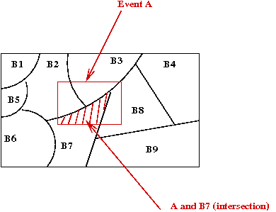
Operations on events:
- The usual set operators apply to events, since events are sets.
- \(A' = \Omega - A\) = complement of \(A\).
- \(A\) and \(B\) = \(A \cap B\) = intersection of event \(A\) and
event \(B\).
Exercise 10:
Use the axioms to show that \(\prob{A'} \eql 1 - \prob{A}\)
for any event \(A\).
Other ways of specifying probability measures:
- For a die-roll, specify as follows:
\(\prob{E} = \frac{|E|}{6}\), for any singleton event \(E\).
- For the die-roll, the singleton events are
$$
\{1\}, \;\;\;\;
\{2\}, \;\;\;\;
\{3\}, \;\;\;\;
\{4\}, \;\;\;\;
\{5\}, \;\;\;\;
\{6\}, \;\;\;\;
$$
- Or, in shorter form, the six events \(\{i\}\) for \(i=1,2,\ldots,6\).
- By assuming (or declaring) that
$$
\prob{\{i\}} \eql \frac{1}{6}
$$
we can build the rest of the probability measure.
- Note: this achieves two purposes
- Compact representation (instead of full list of events).
- Assumes Axiom 3 is satisfied
\(\Rightarrow\) Axiom 3 is used by construction
e.g., \(\prob{\{1,3,5\}} = \prob{\{1\}} + \prob{\{3\}} + \prob{\{5\}} = \frac{1}{6} + \frac{1}{6} + \frac{1}{6} = \frac{3}{6}\)
- Similarly, for a single card drawing:
\(\prob{E} = \frac{|E|}{52}\), for any singleton event
\(E=\{i\}\) (a particular card).
- For a larger subset like \(E'=\{0,1,...,12\}\)
$$\eqb{
\prob{E'} \eqt \prob{\{0,1,\ldots,12\}} \\
\eqt \prob{\{0\}} + \prob{\{1\}} + \ldots + \prob{\{12\}}
\;\;\;\;\;\;\mbox{using Axiom 3} \\
\eqt \frac{1}{52} + \frac{1}{52} + \ldots + \frac{1}{52}\\
\eqt \frac{13}{52}
}$$
- Thus, \(\prob{E'} = \frac{|E'|}{52}\), for any event \(E'\)
- Notation: we will occasionally use an informal event
description (in English) e.g.,
\(\probm{draw a spade} = \frac{13}{52}\).
Simple and complex experiments:
- Consider two die rolls:
- Sample space:
$$\eqb{
\Omega & \eql &
\{(1,1), (1,2), (1,3), (1,4), (1,5), (1,6),\\
& &
(2,1), (2,2), (2,3), (2,4), (2,5), (2,6), \\
& &
(3,1), (3,2), (3,3), (3,4), (3,5), (3,6), \\
& &
(4,1), (4,2), (4,3), (4,4), (4,5), (4,6), \\
& &
(5,1), (5,2), (5,3), (5,4), (5,5), (5,6), \\
& &
(6,1), (6,2), (6,3), (6,4), (6,5), (6,6)\}
}$$
- Thus, there are \(2^{36}\) possible events.
- The convenient way to specify:
\(\prob{E} = \frac{|E|}{36}\), for each single event \(E\).
- For example: \(\prob{(4,3)} = \frac{1}{36}\)
- Then, one can calculate other probabilities.
- Consider the event "same number on both dice".
- This corresponds to the subset (event):
$$ \{(1,1), \;(2,2), \;(3,3), \;(4,4),
\;(5,5), \;(6,6)\}$$
- Which can be written as the union of disjoint singleton
events:
$$
\{(1,1)\} \;\cup\; \{(2,2)\} \;\cup\; \{(3,3)\} \;\cup\; \{(4,4)\}
\;\cup\; \{(5,5)\} \;\cup\; \{(6,6)\}
$$
- Therefore, since \(\prob{\{(i,i)\}} = \frac{1}{36}\) (by assumption)
$$\eqb{
\probm{same number on both dice} & \eql &
\prob{ \{(1,1), \;(2,2), \;(3,3), \;(4,4),\;(5,5), \;(6,6)\} } \\
& \eql &
\prob{ \{(1,1)\} \;\cup\; \{(2,2)\} \;\cup\; \{(3,3)\} \;\cup\; \{(4,4)\}
\;\cup\; \{(5,5)\} \;\cup\; \{(6,6)\} } \\
& \eql &
\prob{\{(1,1)\}} \plss \prob{\{(2,2)\}}, \plss \prob{\{(3,3)\}},
\plss \prob{\{(4,4)\}} \plss \prob{\{(5,5)\}}
\plss \prob{\{(6,6)\}} \\
& \eql & \frac{1}{36} \ops{+} \frac{1}{36}
\ops{+} \frac{1}{36} \ops{+} \frac{1}{36} \ops{+} \frac{1}{36}
\ops{+} \frac{1}{36}\\
& \eql & \frac{6}{36}
}$$
- More complex experiments can be constructed out of simpler ones.
Exercise 11:
Suppose we draw two cards without replacement:
-
What is a compact way of representing the sample space for
two card drawings without replacement? What is the size of the
sample space?
-
What subset corresponds to the event "both are spades"?
- What is the cardinality of this subset?
- What, therefore, is the probability that "both are spades"?
- What is the probability of "first card is a spade"? Work this
out by describing the subset and its cardinality.
Exercise 12:
Consider this experiment: flip a coin repeatedly until you
get heads. What is the sample space?
A minor tweak to Axiom 3:
- Since $$\prob{A \cup B} \eql \prob{A} + \prob{B}$$ it's true
that
$$\prob{A \cup B \cup C} \eql \prob{A} + \prob{B} + \prob{C}$$
- In general,
$$
\prob{A_1 \cup A_2 \cup \ldots \cup A_n}
\eql
\prob{A_1} + \prob{A_2} + \ldots + \prob{A_n}
$$
- But consider a sample space like this:
\(\Omega = \{1, 2, 3, ...\}\) (countably infinite)
- Let event \(A_i=\{i\}\).
- Let event
$$\eqb{
A & \eql & \mbox{ union of all } A_i's \\
& \eql & A_1 \cup A_2 \cup \ldots \\
& \eql & \bigcup_{i=1}^\infty A_i
}$$
- Then, the event \(A\) makes sense and must be accounted for.
- Another example: the event
$$
A' \eql A_1 \cup A_3 \cup A_5 \cup \ldots
$$
(the odd numbers)
- Countable additivity axiom:
$$\eqb{
\prob{A} & \eql & \prob{A_1} + \prob{A_2} + \ldots \\
& \eql & \sum_{i=1}^\infty \prob{A_i}
}$$
Or
$$
\prob{\bigcup_{i=1}^\infty A_i} \eql \sum_{i=1}^\infty \prob{A_i}
$$
\(\Rightarrow\) Axiom 3 needs to hold for countable unions of disjoint events.
The meaning of probability: the frequentist interpretation
- Consider an experiment, an event \(E\) and the number \(\prob{E}\).
- Suppose we are able to repeat the experiment any number of times.
- Let \(f(n) =\) number of times event \(E\) occurs in
\(n\) repetitions (trials).
- Then,
$$
\lim_{n\to\infty} \frac{f(n)}{n} \eql \prob{E}
$$
As it turns out, there is another intepretation, based on the
intuitive term belief
But that needs a little more background (an understanding of distributions)
6.6 Conditional probability
About conditional probability:
- The theory developed so far can be used to solve many simple
word problems.
- However, it does not account for questions of this sort:
Given that the outcome of a die-roll is odd, what then is
the probability that the outcome is \(3\)?
- Unfortunately, there does not seem to be an event
corresponding to the above item of interest.
Consider the die-roll example:
- Define the events
\(A = \{3, 4\}\)
\(B = \{1, 3, 5\}\)
- Suppose we are interested in: what is the probability that \(A\)
occurred given that B occurred?
- Consider \(n\) repetitions of the experiment and let
\(f_B(n) = \) # occurrences of \(B\)
\(f_{AB}(n) = \) # occurrences of \(B\) when \(A\) also occurs
- For example, suppose we performed \(n=7\) trials and
observed these outcomes: \(5, 2, 3, 4, 1, 3, 2\)
- \(f_B(n)\) = 4.
- \(f_{AB}(n)\) = 2.
- Then, for large \(n\),
the desired conditional probability is approximately
$$
\frac{f_{AB}(n)}{f_B(n)}
$$
- Next, divide both sides by \(n\):
$$
\frac{\frac{f_{AB}(n)}{n}}{\frac{f_B(n)}{n}}
$$
- In the limit
$$\eqb{
\frac{f_{AB}(n)}{n} & \;\; \to \;\; & \prob{A \mbox{ and } B} \\
\frac{f_B(n)}{n} & \;\; \to \;\; & \prob{B} \\
}$$
- Thus,
$$
\probm{observe A given B} \eql \frac{\prob{A \mbox{ and } B}}{\prob{B}}
$$
- We write this as
$$
\prob{A | B} \eql \frac{\prob{A \mbox{ and } B}}{\prob{B}}
$$
More formally,
- The conditional probability \(\prob{A|B}\) is defined as
$$
\prob{A | B} \eql \frac{\prob{A \mbox{ and } B}}{\prob{B}}
$$
- It's equally often written as
$$
\prob{A | B} \eql \frac{\prob{A \cap B}}{\prob{B}}
$$
- Note that \([A|B]\) is not an event.
- Read \(\prob{A|B}\) as probability of "A given B".
Exercise 13:
Consider an experiment with three coin flips. What is the
probability that 3 heads occurred given that at least one
occurred?
Exercise 14:
Consider two card drawings without replacement. What is the probability
that the second card is a club given that the first is a club?
An important variation of stating the rule for conditional probability:
- Recall the definition:
$$
\prob{A | B} \eql \frac{\prob{A \cap B}}{\prob{B}}
$$
- By re-arranging the definition
$$
\prob{A|B} \; \prob{B} \eql \prob{A \cap B}
$$
- By symmetry,
$$
\prob{B|A} \; \prob{A} \eql \prob{A \cap B}
$$
- Thus, for any two events \(A, B\):
$$
\prob{A|B} \; \prob{B} = \prob{B|A} \; \prob{A}
$$
An interesting twist:
- Notice that we can re-arrange the last equation as
$$
\prob{A|B} \eql \frac{\prob{B|A} \; \prob{A}}{\prob{B}}
$$
- Next, consider the card example (without replacement):
- Let \(A = \) first card was a club.
- Let \(B = \) second card was a club.
- Then, \(\prob{A|B} = \) probability first was a club
given that the second was a club.
- Thus, it seems as though we can reason about past events
given knowledge of current events.
- This is strictly not true, because the sample space consists
of the entire history (for two card drawings):
\(\Omega\) =
{(0,1),...,(0,51),
(1,0), (1,2)...,(1,51),
...
(51,0), (51,2)...,(51,50)}
Thus, we are really reasoning about the entire history.
- This idea
$$
\prob{A|B} \eql \frac{\prob{B|A} \; \prob{A}}{\prob{B}}
$$
is often called Bayes' rule.
Back to the card problem:
- Recall the earlier problem:
- The probability that the first card is a club given
that the second is a club.
- The probability that the first card is a diamond given
that the second is a club.
- Define these events:
\(C_1 = \) first card is a club
\(C_2 = \) second card is a club
\(D_1 = \) first card is a diamond
- Then,
$$
\prob{C_1 | C_2} \eql
\frac{\prob{C_2 | C_1} \; \prob{C_1}}{\prob{C_2}}
$$
- Observe that
$$\eqb{
\prob{C_1} & \eql & \frac{13}{52} \\
\prob{C_2} & \eql & \frac{13}{52} \\
\prob{C_2 | C_1} & \eql & \frac{12}{51}
}$$
Exercise 15:
Why? Explain by describing the events \(C_1\) and \(C_2\) as subsets
of the sample space and evaluating their cardinalities (sizes).
- Substituting, we get \(\prob{C_1 | C_2} = \frac{12}{51}\).
Exercise 16:
What is \(\prob{D_1}\)?
Compute \(\prob{D_1 | C_2}\).
A variation of Bayes' rule:
- Recall that
$$
\prob{A \cap B} \eql \prob{A|B} \; \prob{B}
$$
- Suppose the sample space can be partitioned into disjoint
sets \(B_1, B_2, \ldots, B_n\) such that
- The \(B_i\)'s are disjoint.
- \(\Omega = \) union of the \(B_i\)'s.
- Then, for any event \(A\), the events
\(A \cap B_1\),
\(A \cap B_2\),
\(\vdots\)
\(A \cap B_n\)
are all disjoint.
- And, just as importantly
$$
A \eql (A\cap B_1) \cup (A\cap B_2) \cup \ldots \cup (A\cap B_n)
$$
- Thus,
$$\eqb{
\prob{A}
& \eql & \prob{(A\cap B_1) \cup (A\cap B_2) \cup \ldots \cup (A\cap B_n)}\\
& \eql & \prob{(A\cap B_1)} + \prob{(A\cap B_2)} + \ldots + \prob{A\cap B_n)}\\
& \eql &
\prob{A | B_1} \; \prob{B_1} \plss
\prob{A | B_2} \; \prob{B_2} \plss
\; \ldots \;
\prob{A | B_n} \; \prob{B_n}
}$$
This is sometimes called the law of total probability
- Example: two cards are drawn without replacement. What is
the probability the second card is an ace?
Let \(A = \) second card is an ace.
Let \(B = \) first card is an ace.
Then, \(B\) and \(B'\) form a partition.
Then, \(\prob{A} \eql \prob{A|B} \; \prob{B} \plss
\prob{A|B'} \; \prob{B'}\)
Exercise 17:
Finish (by hand) the calculation above.
Consider another example:
- A lab performs a blood test to reveal the presence or absence
of a certain infection.
- The test is not perfect
\(\Rightarrow\) If a person is infected, the test may not always work.
\(\Rightarrow\) An uninfected person may have a test turn out positive (false positive).
- Assume we have the following model:
- 5% of the population is infected.
- The probability that the test works for an infected person
is 0.99.
- The probability of a false positive is 3%.
- We want the following probabilities:
- Probability that if a test is positive, the person is
infected.
- Probability that if a test is positive, the person is well.
- Define these events:
\(S = \) person is sick
\(T = \) test is positive
Exercise 18:
Write down the desired probabilities in terms of what's given
in the model, and complete the calculations.
Write a program to confirm your calculations:
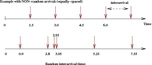
6.7 Continuous sample spaces
Consider the following example:
Exercise 19:
Download and execute BusStopExample.java.
You will also need BusStop.java.
- What is \(Pr[A \gt 1]\)? What is \(Pr[A \gt 0.5]\)?
- What is an example of an event for the above sample space?
- Is \(\{1.0, 1.2, 1.5\}\) an event?
- Is the interval \([1.0, 3.5]\) an event?
Exercise 20:
Change the type of interarrival by replacing
true
with false above, and
estimate both \(\prob{\mbox{first-interarrival } \gt 0.5}\) and
\(\prob{\mbox{first-interarrival } \gt 1}\).
Note: using
true
results in using \(exponential\) interarrivals and using
false
results in using \(uniform\) interarrivals. We'll understand later
what these mean.
Exercise 21:
Modify the code to estimate the following conditional
probability. Let \(A\) denote the interarrival time.
Estimate \(\prob{A \gt 1.0 | A \gt 0.5}\) for each of
the two types of interarrivals (exponential and uniform).
What is strange about the result you get for
the exponential type?
Hint: compare this estimate to that in the previous exercise;
that is, compare \(\prob{A \gt 1.0 | A \gt 0.5}\)
with \(\prob{A \gt 0.5}\). What is the implication?
Exercise 22:
Estimate the average interarrival time for each
of the two types of interarrivals (exponential and uniform).
More on the same example:
- Suppose we arrive at the bus stop at time=10.0.
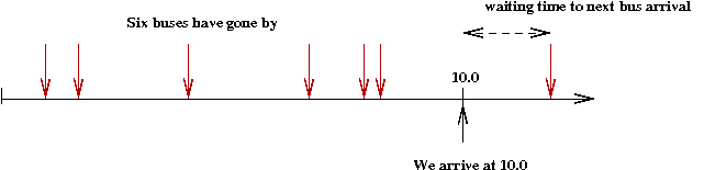
- We can count how many buses have gone by:
(source file)
        double myArrivalTime = 10;                    // We arrive at 10.0
        BusStop busStop = new BusStop (true);
        double arrivalTime = 0;
        double numBuses = -1;
        while (arrivalTime < myArrivalTime) {
            numBuses ++;
            busStop.nextBus ();                       // Keep generating successive buses
            arrivalTime = busStop.getArrivalTime ();
        }
        System.out.println ("Number of buses: " + numBuses);
Exercise 23:
Why doesn't the following code work?
        ...
        double numBuses = 0;
        while (arrivalTime < myArrivalTime) {
            busStop.nextBus ();
            arrivalTime = busStop.getArrivalTime ();
            numBuses ++;
        }
        ...
Exercise 24:
Modify the above program
to estimate the probability
that at least 5 buses have gone by.
Exercise 25:
Consider the waiting time: the time from your arrival
(at 10.0) to the time the next bus arrives.
Estimate your average waiting time.
- Does this depend on when you arrival (at 10.0 vs. 20.0, for example)?
- Try this for each of the two types of interarrivals
(exponential and uniform).
- What do you observe is unusual about this wait time?
6.8 (In)Dependence
Consider flipping a coin twice:
- Let \(C_1\) be the event: "first flip is heads"
- Let \(C_2\) be the event: "second flip is heads"
- We will compute \(\prob{C_2}\)
and \(\prob{C_2 | C_1}\).
- Here is a simple program to estimate both:
(source file)
	double numTrials = 1000000;

	double numSuccesses = 0;                   // #times C2 occurs.
        double numFirstHeads = 0;                  // #times C1 occurs.
        double numBothHeads = 0;                   // #times both are heads.

	for (int n=0; n<numTrials; n++) {
            Coin coin = new Coin ();

	    int c1 = coin.flip ();
	    int c2 = coin.flip ();

            if (c2 == 1) {
		numSuccesses ++;
            }

            if (c1 == 1) {
                numFirstHeads ++;
                if (c2 == 1) {
                    numBothHeads ++;
                }
            }
	}

        double prob1 = numSuccesses / numTrials;           // Pr[C2]
        double prob2 = numBothHeads / numFirstHeads;       // Pr[C2|C1]

	System.out.println ("Pr[c2=1]=" + prob1 + "  Pr[c2=1|c1=1]=" + prob2);
Exercise 26:
Instead of Coin.java in the example
above, use BizarreCoin.java
and see what you get.
Some definitions:
- Two events \(A\) and \(B\) are independent
if \(\prob{A|B} = \prob{A}\).
- Thus, events \(A\) and \(B\) are dependent
if they are not independent.
- Think of (in)dependence as
"if you know A occurred, does that change the calculation
of the probability of B?"
- Alternatively, "if you know the probability
of A, does it impact the probability of B?"
- Dependence is NOT solely "if A occurred, then B must occur"
(although that is an extreme form of dependence).
Recall that
$$
\prob{A|B} \eql \frac{\probm{A and B}}{\prob{B}}
\eql \frac{\prob{A \cap B}}{\prob{B}}
$$
Thus, if they are independent
$$
\frac{\probm{A and B}}{\prob{B}} \eql \prob{A}
$$
Or,
$$
\probm{A and B} \eql \prob{B} \; \prob{A}
$$
This is how some books define independence.
Exercise 27:
For the bus-stop problem, define the following events:
- Event \(B_1\) = exactly one bus arrives in the period \([0,0.5]\).
- Event \(B_2\) = exactly one bus arrives in the period \([0.5,1]\).
First, without writing a program, what does your intuition tell you
about whether these events are independent?
Next, write a program to estimate \(\prob{B_2}\) and
\(\prob{B_2 | B_1}\).
Do this for each of the exponential and uniform cases.
6.9 Problem solving
Probability problems are often tricky and defy intuition.
We suggest the following high-level
problem-solving procedure:
- Identify the sample space and find some compact way of writing
it down.
- Identify the question being asked:
- Is it an event (subset of the sample space)?
- Or is it a conditional probability?
- Is conditioning involved? That is, does it seem
like one action will change the probabilities for a later action?
\(\Rightarrow\) If so, the conditional probabilities are usually
easier to read off from the problem.
- Identify relevant events and write them down, if possible,
as subsets of the sample space.
- Try to identify, if conditioning is involved, which
conditional probabilities are useful.
- How is the probability measure specified?
- Finally, complete the calculations, simplifying
fractions only near the end.
Let's look a simple example: what is the probability that
a rolled pair of dice shows the same number?
- Identify the sample space:
\(\{(i,j): i,j \in 1,2,...,6\}\)
- There appears to be no conditioning.
- The event of interest:
Let \(A = \{(i,i): i \in 1,2,...,6\}\)
- The probability measure is not specified.
We'll make the assumption that each singleton event is equally likely.
- Now we solve the problem:
\(\prob{A} = \frac{|A|}{|\Omega|} = \frac{6}{36}\)
Let's look a little deeper at the above problem:
- A more intuitive measure is: each number shows up with equal
probability on each die
\(\prob{i} = \frac{1}{6}\), \(i \in \{1,...,6\}\)
- This is what we had assumed earlier as probabilities
for singleton events.
- How does this give us
\(\prob{(i,j)} = \frac{1}{36}\), \(i,j \in \{1,...,6\}\)?
- Define the events
\(A_i\) = "obtain i on first roll"
\(B_j\) = "obtain j on second roll"
- Then, one can assume independence (because the second roll
shouldn't be affected by the outcome of the first):
\(\prob{A_i} = \frac{1}{6}\)
\(\prob{B_j} = \frac{1}{6}\)
- Therefore,
\(\prob{(i,j)} = \prob{A_i}\prob{B_j} = \frac{1}{36}\)
- Thus, the assumption of independence is buried when we state
\(\prob{A} = \frac{|A|}{|\Omega|}\)
for this example.
Another example:
Let's now look at an instructive variation of the above:
Exercise 28:
Three subcontractors - let's call them \(A,B,C\) - to a popular
clothing store contribute roughly
20%, 30% and 50% of the products in the store.
Turns out that 6% of \(A\)'s products have some defect; the defect numbers
for \(B\) and \(C\) are 7% and 8% respectively.
A product is selected at random and found to be defective. What
is the probability that it came from subcontractor \(A\)?
Exercise 29:
We have seen four key examples: a coin, a die, a deck of cards,
and the bus-stop. Examine the code in each of:
Coin.java,
Die.java,
CardDeck,
and
BusStop.java.
See if you can make sense of how random outcomes are created.
(There's no written answer required for this question.)
© 2008, Rahul Simha