\(
\newcommand{\blah}{blah-blah-blah}
\newcommand{\eqb}[1]{\begin{eqnarray*}#1\end{eqnarray*}}
\newcommand{\eqbn}[1]{\begin{eqnarray}#1\end{eqnarray}}
\newcommand{\bb}[1]{\mathbf{#1}}
\newcommand{\mat}[1]{\begin{bmatrix}#1\end{bmatrix}}
\newcommand{\nchoose}[2]{\left(\begin{array}{c} #1 \\ #2 \end{array}\right)}
\newcommand{\defn}{\stackrel{\vartriangle}{=}}
\newcommand{\rvectwo}[2]{\left(\begin{array}{c} #1 \\ #2 \end{array}\right)}
\newcommand{\rvecthree}[3]{\left(\begin{array}{r} #1 \\ #2\\ #3\end{array}\right)}
\newcommand{\rvecdots}[3]{\left(\begin{array}{r} #1 \\ #2\\ \vdots\\ #3\end{array}\right)}
\newcommand{\vectwo}[2]{\left[\begin{array}{r} #1\\#2\end{array}\right]}
\newcommand{\vecthree}[3]{\left[\begin{array}{r} #1 \\ #2\\ #3\end{array}\right]}
\newcommand{\vecdots}[3]{\left[\begin{array}{r} #1 \\ #2\\ \vdots\\ #3\end{array}\right]}
\newcommand{\eql}{\;\; = \;\;}
\newcommand{\dv}[2]{\frac{#1}{#2}}
\newcommand{\half}{\frac{1}{2}}
\newcommand{\mmod}{\!\!\! \mod}
\newcommand{\ops}{\;\; #1 \;\;}
\newcommand{\implies}{\Rightarrow\;\;\;\;\;\;\;\;\;\;\;\;}
\definecolor{dkblue}{RGB}{0,0,120}
\definecolor{dkred}{RGB}{120,0,0}
\definecolor{dkgreen}{RGB}{0,120,0}
\)
Module 5: Robotics Interlude - Reactive Control
5.1 PID Control
Exercise 1:
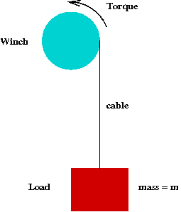
Recall the winch example: Winch.java.
Try different torque (voltage) values to lift the load to the desired
height. You will also need
Function.java and
SimplePlotPanel.java.
Upon clicking "stop" you will see how the distance y varies with time.
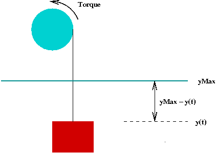
Consider the control problem in the winch example:
- We would like to set the torque at various times so
that the load reaches the target height.
\(\Rightarrow\)
The top of the load should align with the target line.
- Ideally, we should go towards the target quickly and
slow down as it nears the target
\(\Rightarrow\)
As in an elevator.
- Ideally, we would prefer not to overshoot the target.
- We will add one minor twist:
- Typically, motors are controlled through voltage supplied
\(\Rightarrow\)
We'll make the simple assumption that torque is proportional to voltage
- Henceforth, we will control voltage.
Consider two broad approaches to control:
- Fully pre-computed control:
- Compute a voltage function \(V(t)\) ahead of time and apply it.
\(\Rightarrow\)
At each time step \(t\), set the voltage to \(V(t)\).
- The function should take us directly to our desired goal
\(\Rightarrow\)
This approach is roughly equivalent to planning.
- To find such a function, we would have to (efficiently) search the
space of all possible such functions.
\(\Rightarrow\)
We did something similar for the car-acceleration problem.
- Adjust-as-you-go (reactive) control:
- Use sensor readings to estimate current position.
- Update control based on current position and desired position.
We'll focus on the latter approach in the winch problem:
- The desired position is given by yMax
- At any given moment, the current position is y
- One simple idea: proportional control:
- Key idea: the further away we are, the larger the torque.
- Let \(V(t) = k_P \; (y_{Max} - y(t))\).
- The minus sign matters!
- Note: we only need the current position \(y(t)\) at any
given time to set the voltage at that time.
Exercise 2:
Implement proportional control for the horizontal case
in the nextStep()
method of Winch2.java.
Experiment with different values of the constant \(k_P\),
for example: \(k_P=50,500.\)
What do you observe? Where have you seen this dynamic behavior before?
What is the value of
yMax
in the code?
What would happen if we mistakenly set the voltage
to \(V(t) = k_P \; (y_{Max} + y(t))\)? Try to reason this out
before implementing.
To address the above problem, we will use damping:
- Note: we want the speed at yMax to be zero.
\(\Rightarrow\)
We want to reduce the rate of change as we approach the target (yMax).
- We will include a damping term to the control:
- Let \(V(t) = k_P (y_{Max} - y(t)) - k_D y'(t) \).
- Intuition: if the rate of change in \(y(t)\) is high,
reduce the voltage.
- This combination is called proportional-derivative control.
Exercise 3:
Implement proportional-derivative control
for the horizontal case
in Winch3.java.
Experiment with different values of the constants \(k_P\)
and \(k_D\).
For example: \(k_D=10, 100, 1000\) (using previous
values of \(k_P=50,500\)).
Does any value of \(k_D\) fix the problem?
Exercise 4:
Apply PD-control to the vertical case,
writing that version in
Winch4.java.
Again, experiment with different values of
\(kP\). What do you observe?
To address the above problem, we will use integrative-control:
- The problem is that \(V(t) = 0\) when \(y=y_{Max}\) and
\(y'(t)=0\)
\(\Rightarrow\)
But at least some torque is needed to hold the load (under gravity)
\(\Rightarrow\)
Cannot have \(V(t)\) settle to zero.
- If we knew the final desired torque
\(\Rightarrow\)
We could set that torque directly
- Unfortunately, this depends on load (which we can't predict)
\(\Rightarrow\)
We would like an approach independent of load
- Key ideas with integrative-control:
- Allow torque to build up to a finite value.
- Use an infinite sum of terms.
\(\Rightarrow\)
Terms should get smaller as you approach target
- Define
$$\eqb{
S(t) & \eql & S (t-\Delta t) + (y_{Max} - y(t)) \\
& \eql & \mbox{ accumulated differences}
}$$
- Let
$$
V(t) = k_P (y_{Max} - y(t)) - k_D y'(t) + k S(t).
$$
- Why is this called integrative-control?
- We can make the sum \(S(t)\) a true integral (of the error):
$$
S(t) \eql S(t-\Delta t) + \Delta t(y_{Max} - y(t))
$$
- Then, define
$$
V(t) \eql k_P (y_{Max} - y(t)) - k_D y'(t) + k_I S(t)
$$
- The \(\Delta t\) term, however, can be absorbed into the
constant \(k_I\).
- The combination of proportional, derivative and integral
control is called PID control.
Exercise 5:
Apply PID-control to the vertical case,
writing your code in
Winch5.java.
Experiment with different \( k_I\) values.
5.2 Reactive vs planned control
In planned control:
- We have advance knowledge of the goal and everything in between.
- Given this, we can compute a sequence of steps to get from
the "start" to the "goal"
\(\Rightarrow\) This was the approach taken by planning algorithms
- Example: the arm control problem.
- Example: the car acceleration problem
- In this case, we constructed an entire acceleration function.
- The goal: the acceleration function was applied to take
a vehicle from start to finish in as little time as possible.
Contrast this with reactive control:
- In the winch problem, the only information used was the
distance to the goal.
- The algorithm
- Used the difference as input to the control (voltage, in
that example).
- Used its own estimate of derivative/integral for PID control.
Can a reactive approach be used in a robot planning problem?
- Consider a robot navigation problem.
- Suppose we only know the goal's coordinates
(And no knowledge of obstacles.)
- The robot has sensors and must react to input from the sensors.
We will consider simple range sensors:
- Here, a robot has \(N\) range sensors equally spaced
in a circle.
- Thus, if \(N=8\), the robot can sense distance
in 8 directions (N,S,E,W, NE,NW,SE,SW) relative to its orientation.
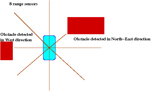
- We will assume that the sensor returns the distance
to the closest obstacle in each sense-direction.
- The most common (and least expensive) type of range sensor: sonar.
- Note: we will use the convention that North is the direction
the vehicle is facing (and thus, changes all the time).
Exercise 6:
Download and unpack carSim.jar.
Use java CarGUI manual on the command-line to run in
manual mode, then select the Unicycle and "basic sensor".
Drive around some obstacles (scene-3 or scene-4) and observe
how the sensors work.
Exercise 7:
Examine the file BasicSensorPack.java. You can access
the variable sonarDistance[] to get these distances.
Here, sonarDistance[0] is the distance in front (North
of the vehicle).
Next, use this template to
write a simple car controller for Scene-3 that goes
towards the obstacle, stops just before it and turns left to face
North. Don't forget to select "Basic sensor" in carGUI
when testing.
Next, we will try and follow the "wall" and wind our
way around the obstacle:
- We will circumnavigate obstacles by going clockwise
\(\Rightarrow\) turn left when close enough
- After turning so that we're parallel to the wall, we will
move forward.
- In moving forward, we will:
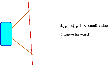
- Examine the NE and SE sensor readings.
- Try to keep these the same.
- Thus, if the NE distance is larger, turn right (slightly):
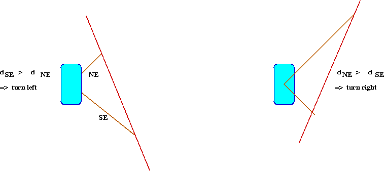
- Thus, if the SE distance is larger, turn left (slightly).
- If the distances are approximately the same, move forward:
- If, when moving forward, we're too close to an obstacle,
turn left.
- In pseudocode:
       1.   while true
       2.       if |dNE - dSE| < α
       3.           if dN > δ
       4.               move forward
       5.           else
       6.               stop and turn left
       7.           endif
       8.       else if dNE > dSE
       9.           stop and turn right
       10.      else
       11.          stop and turn left
       12.      endif
       13.  endwhile
- Which can be shortened to (and leaving out the loop):
       1.   if |dNE - dSE| < α and dN > δ
                // Approximately parallel to wall, and no obstacle in front.
       2.       move forward
       3.   else if dNE > dSE
       4.       stop and turn right
       5.   else
       6.       stop and turn left
       7.   endif
Exercise 8:
Implement the above algorithm in your controller using
\(\alpha=10, \delta=40\) and a forward velocity of 10,
with Scene-3 as the setting.
The NE distance is sonarDistance[7] whereas
the SE distance is sonarDistance[5] (going anti-clockwise).
Recall that we need to set the steering angle \(\phi\gt 0\) to turn
left and \(\phi\lt 0\) to turn right.
What do you notice when the unicycle tries to turn right
at the obstacle corner?
To address the problem:
- We will include some forward motion:
       1.   if |dNE - dSE| < α and dN > δ
       2.       move forward
       3.   else if dNE > dSE
       4.       reduce speed and turn right
       5.   else
       6.       reduce speed and turn left
       7.   endif
- This way, we will not repeat a position and get stuck.
Exercise 9:
Implement the above algorithm in your controller.
Use vel=2 as the reduced speed. Does it solve the problem?
Next, let us use the PID approach:
- Notice that \(d_{NE} - d_{SE}\) determines
our action:
- If \(|d_{NE} - d_{SE}| \approx 0\)
\(\Rightarrow\) No turn (\(\phi=0\))
- If \(d_{NE} - d_{SE} \gt 0\)
\(\Rightarrow\) right turn (\(\phi\lt 0\)
- If \(d_{SE} - d_{NE} \gt 0\)
\(\Rightarrow\) left turn (\(\phi\gt 0\))
- Thus, we can summarize this as
amount of left turn = \(d_{SE} - d_{NE}\)
- Define
$$\eqb{
e(t) & \eql & (d_{SE} -d_{NE}) \\
& \eql & \mbox{ difference at time } t
}$$
- Then, proportional control (at any time \(t\))
can be described as:
$$
\phi \eql k_P e(t)
$$
where \(\phi\) is the left-turn steering angle.
- In pseudocode
       1.   if |dNE - dSE| < α and dN > δ
       2.       move forward
       3.   else
       4.       reduce speed
       5.       set φ = kP e(t)
       6.   endif
Exercise 10:
Implement proportional control in your controller. Use a small
(e.g. vel=2) velocity throughout. Experiment with
different values of the proportionality constant \(k_P\).
What do you observe when the vehicle turns a corner?
To damp out the oscillations, let's use differential control:
- We will store the previous value of \(e(t)\) (at time
\(t'\)) and estimate
$$
e'(t) \eql \frac{e(t) - e(t')}{t - t'}
$$
- Then define the control
$$
\phi \eql k_Pe(t) - k_De'(t)
$$
Exercise 11:
Add derivative control to your controller.
Experiment with
different values of the two proportionality constants
\(k_P\)
and
\(k_D\)
What do you observe?
Bounds on values:
- Sometimes, the difference or differential term in PD control
can get very large.
- One simple solution is to bound sensor values, e.g.
if \( d_{NE} \gt 2 d_{SE}\), then
set \( d_{NE} = 2 d_{SE}\)
Exercise 12:
See if bounding the sensor values (as inputs to
the algorithm) makes a difference. Observe what
happens as the vehicle turns near the third obstacle
corner (near the x-axis, as it's headed down).
An additional fix:
- We need to make sure we keep a safe distance from the wall.
- To do this, we could read the East-sensor
\(\Rightarrow\) identify the distance looking rightwards
- Key idea: if it's too close (less than distance \(δ\)),
turn left (away from wall).
- Pseudocode:
       Algorithm: follow-wall
       1.   if dE < δ
       2.       reduce speed and turn left
       3.   else if |dNE - dSE| < α and dN > δ
       2.       move forward
       3.   else
       4.       reduce speed
       5.       set φ = kP e(t) - kD e'(t)
       6.   endif
Exercise 13:
Implement the above algorithm and see if it works.
Can you suggest improvements?
5.3 State-based control
Now let's return to our original problem of getting the vehicle
to a desired destination:
- Assumptions:
- Destination coordinates are known.
- Nothing is known about obstacles.
- We will have readings from the 8 range sensors at any time.
- A simple algorithm:
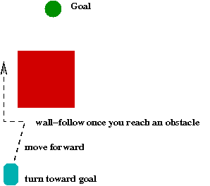
- Head towards goal
\(\Rightarrow\) We can do this because we can compute the angle towards
the goal
- If an obstacle is encountered, use wall-following to
go around the obstacle
- Some notation:
\(\theta \) = current orientation (heading)
\(\gamma \) = direction to goal
- Pseudocode:
      Algorithm: goal-seek
      1.   if dN > δ and |θ-γ| > ε
               // There's no obstacle, but we're not in the right direction.
      2.       turn towards goal
      3.   else if dN > δ and |θ-γ| < ε
               // We're in the right direction, and there's no obstacle.
      4.       move forward
      5.   else
      6.       follow-wall        // As in previous section.
      7.   endif
Exercise 14:
Implement the above in
MySimpleCarController2.java
and see if it works. What do you observe?
To address this problem:
- We need to give "turning" enough time.
\(\Rightarrow\) We need to stay "in turning mode" for a while.
\(\Rightarrow\) Need state-based control.
- Key ideas in state-based control:
- Know which "state" you are in.
- In each state, apply appropriate control.
- Let's try this out:
     1.   if state = Turn-To-Goal
     2.       φ = kP (γ - θ)            // Turn towards goal.
     3.       if γ - θ < ε
     4.           state = Move-Forward  // Change state if direction is correct
     5.       endif
     6.   else if state = Move-Forward
     7.       if dN > δ and |θ-γ| < ε
     8.           move-forward
     9.       else
     10.          follow-wall           // As in the previous section.
     11.      endif
     12.  endif
Exercise 15:
Implement the above algorithm and see if it works.
Re-seeking the goal:
- When wall-following, we could potentially turn away from the
goal
\(\Rightarrow\) We need to keep looking to see if we can get to the goal.
- Key ideas:
- While wall-following, see if we have line-of-sight to goal.
- Since we don't have line-of-sight, we'll use an approximation:
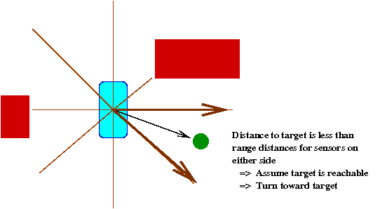
- Pseudocode:
     1.   if state = Turn-To-Goal
     2.       φ = kP (γ - θ)            // Turn towards goal.
     3.       if γ - θ < ε
     4.           state = Move-Forward  // Change state if direction is correct
     5.       endif
     6.   else if state = Move-Forward
     7.       if dN > δ and |θ-γ| < ε
     8.           move forward
     9.       else
     10.          follow-wall           // As before.
     11.      endif
     12.      if open-to-goal
     13.          state = Turn-To-Goal
     14.      endif
     12.  endif
Exercise 16:
Implement the above in
MySimpleCarController3.java
and see if it works.
The open-to-goal test has been implemented for you.
Exercise 17:
How can you determine whether it's closer to turn clockwise
vs. anticlockwise?
Exercise 18:
What happens if we are too close to an obstacle on the left side?
What changes are needed for obstacle avoidance on the left?
Exercise 19:
Assuming obstacle avoidance works, draw on paper a scenario
on paper where the above goal-seeking algorithm fails to reach
the goal. Suggest a better algorithm.
5.4 Further info
About control theory:
- We have only superficially covered a single problem in
control theory.
- Control theory is a vast subject with many results.
- Linear control theory (including PID).
- Non-linear control theory.
- Stochastic control theory.
- Where is control-theory applied in robotics?
- Simple control theory is useful in optimizing motion.
e.g., optimal turning for Dubin car (single turn)
- Advanced control theory is useful in understanding
fundamental limitations in control (e.g., PD-control vs. PID-control)
Controlling a robot is more than just control theory:
- At the highest level, there's planning (e.g., the A* algorithm):
- Planning takes a distant goal and tries to, using knowledge
from sensors/data etc, create a path.
- Example: various configurations in folding a multi-link arm.
- Executing a plan requires maneuvers in small steps between
various steps:
- A control algorithm enhanced with PID can create smooth
maneuvers.
- Sometimes, the controls depend on the "state",
as we've seen in the above examples.
© 2008, Rahul Simha