\( \newcommand{\blah}{blah-blah-blah} \newcommand{\eqb}[1]{\begin{eqnarray*}#1\end{eqnarray*}} \newcommand{\eqbn}[1]{\begin{eqnarray}#1\end{eqnarray}} \newcommand{\bb}[1]{\mathbf{#1}} \newcommand{\mat}[1]{\begin{bmatrix}#1\end{bmatrix}} \newcommand{\nchoose}[2]{\left(\begin{array}{c} #1 \\ #2 \end{array}\right)} \newcommand{\defn}{\stackrel{\vartriangle}{=}} \newcommand{\rvectwo}[2]{\left(\begin{array}{c} #1 \\ #2 \end{array}\right)} \newcommand{\rvecthree}[3]{\left(\begin{array}{r} #1 \\ #2\\ #3\end{array}\right)} \newcommand{\rvecdots}[3]{\left(\begin{array}{r} #1 \\ #2\\ \vdots\\ #3\end{array}\right)} \newcommand{\vectwo}[2]{\left[\begin{array}{r} #1\\#2\end{array}\right]} \newcommand{\vecthree}[3]{\left[\begin{array}{r} #1 \\ #2\\ #3\end{array}\right]} \newcommand{\vecdots}[3]{\left[\begin{array}{r} #1 \\ #2\\ \vdots\\ #3\end{array}\right]} \newcommand{\eql}{\;\; = \;\;} \newcommand{\eqt}{& \;\; = \;\;&} \newcommand{\dv}[2]{\frac{#1}{#2}} \newcommand{\half}{\frac{1}{2}} \newcommand{\mmod}{\!\!\! \mod} \newcommand{\ops}{\;\; #1 \;\;} \newcommand{\implies}{\Rightarrow\;\;\;\;\;\;\;\;\;\;\;\;} \newcommand{\prob}[1]{\mbox{Pr}\left[ #1 \right]} \newcommand{\expt}[1]{\mbox{E}\left[ #1 \right]} \newcommand{\probm}[1]{\mbox{Pr}\left[ \mbox{#1} \right]} \newcommand{\simm}[1]{\sim\mbox{#1}} \definecolor{dkblue}{RGB}{0,0,120} \definecolor{dkred}{RGB}{120,0,0} \definecolor{dkgreen}{RGB}{0,120,0} \)

Module 11: Machine Learning

11.1 What is machine learning?

The "machine" part is easy to understand: algorithms.

What about the "learning" part?

Broadly, one could say: we're interested in software that improves "performance" over time.

Consider a gradient-descent optimization algorithm: is it learning?

In some senses, yes, because it's learning something about the function as it drives towards the optimum.
But one could say that its "job" is to find the optimum
$\Rightarrow$ Its ability to do so does NOT improve with successive trials or with new functions.
$\Rightarrow$ We don't consider this learning.

An optimization algorithm that performs better and better as it encounters more functions?
$\Rightarrow$ Yes, we would say some "learning" is going on.

At the very least, it looks like a learning algorithm will need to store "experience" in some way.

We will focus on a particular kind of machine learning problem
$\Rightarrow$ The classification problem

Before that, let's look at some motivating examples.

Exercise 1: Can you find an example of an application on the web that learns?

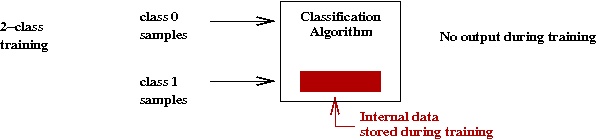
Meet our example (classification) applications:

All of the data will lie in two classes (for simplicity of presentation).
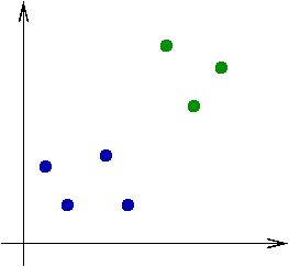
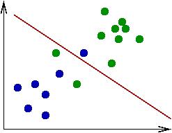
Classifying 2D points:
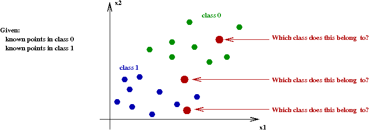
- We're given some already-classified data (blue, green points).
- The data here are in two classes (categories, groups, whatever).
- For a new point, we need to decide which class the point belongs to.
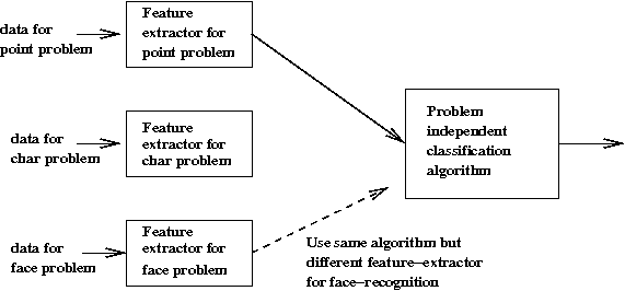
Classifying handwritten characters:
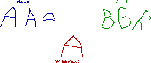
- The input: samples of already-classified data (chars from each of the classes).
- For a newly-written char, which class does it match?
Face recognition:
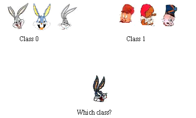
- The input: a set of training images for each class.
- For a new image, which class does it belong to?

Exercise 2: Download and unpack classifier.jar. Then inside the classifierJar directory, execute ClassifierGUI.

In the Point-problem, generate some points to see where the two classes fall. Why is the split-uniform data set harder (from a machine-learning viewpoint) than the uniform one?
In the Char-problem, click on "load" to load samples of "A" and "B" renderings.
In the Face-problem, click on "load" and browse variety of face samples. Which person shows more variety in images?

Let's try and frame the classification problem more carefully:

First, there are two phases:
- Phase I: training, in which labelled data are given to the algorithm.
- Phase II: testing, or deployment, in which unlabelled data are given, and the goal is to classify them.
How does one evaluate an algorithm?
$\Rightarrow$ We'd like something like: "99% of the test samples were correctly classified."
At first glance, it may seem that very different algorithms would be needed for the three problems.
This is only partly true, as it turns out:
- We will separate the algorithm into two components:
- A feature extractor that is problem-dependent.
- A learning algorithm that is problem-independent.
Let's look at the input to the learning algorithm:
Each input sample is a point in $d$-dimensional space.
Point-problem example:
- Each sample is 2-dimensional (a point): $(x_1, x_2)$.
- The above example has 7 training samples, and one test sample
  $\Rightarrow$ Each of these has dimension = 2.
- During training, all the pre-classified (labelled) data is given to the algorithm.
  $\Rightarrow$ No output during this time.
- During testing, the test sample is given, and the algorithm is expected to classify it.

Thus, a classification algorithm will have methods that look like this:

public interface Classifier {

    // This method is called to supply the algorithm with training
    // data. This is where the "training" is performed.

    public String train (int numClasses, ArrayList<Vector<Double>>[] trainingData);


    // This method is called (perhaps repeatedly) with a test
    // sample. Note that the output is the label (which class the test
    // sample has been found to belong to).

    public int classify (Vector<Double> sample);
}

First look at a single sample above (in the method classify()):
- This is an instance of Vector<Double>.
- Thus, one could examine individual $x_i$'s:
```
       double x_i = sample.get(i);
       System.out.println (x_i);     // Print x_i.
       
```
How is the training data organized?
- Observe that each class has many samples
  $\Rightarrow$ trainingData[c] is the set of samples for class $c$.
- Since one sample is an instance of Vector<Double>
  $\Rightarrow$ A collection of these is used for each class.
- The above example uses an ArrayList for this purpose.
- Thus, ArrayList<Vector<Double>> is a list of samples.
- Finally, there's one of these for each class, hence the array.

Exercise 3: For the point problem:

Create 10 training points from one of the distributions.
Compile and upload the NullClassifier and click the "train" button.

Next, examine the code in NullClassifier. How does the screen output correspond to the generated data?

Exercise 4: Consider the char problem:

How would the data for a single char be represented as as an $d$-dimensional point?
Examine the code in CharProblem.java and identify the manner by which the samples are constructed from line-segments. Where in the code is this being done?
Find a place in the code to print out the dimension $d$ for each test sample (which you create on the right side). What is a typical value of $d$? What kind of character data will have large $d$?

Exercise 5: Similarly, what is the size of $d$ for the face problem? Add code to FaceProblem.java to print out these sizes. Is $d$ the same for all samples?

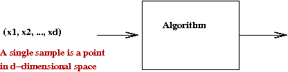
More notation:

We've seen that the dimension $d$ can be quite large in a data set.
Each sample is a point in d-dimensional space
$\Rightarrow$ $(x_1,x_2, ..., x_d)$
- Here, each $x_i$ is a real number
  $\Rightarrow$ the coordinate in dimension $i$.
We will use the shorthand $x = (x_1,x_2, ..., x_d)$.
Note: in some problems, every sample may not have the same dimension
$\Rightarrow$ We have to be prepared to work with different dimensional samples.

Exercise 6: Which of the three applications we've seen has this problem?
$\Rightarrow$ In this case, we may want to pre-process the data to make all samples have the same dimension.
Assume we are given $M$ training samples.
- We'll use the notation $x^{(m)}$ to denote the $m$-th sample.
- Thus, $x_i^{(m)}$ denotes the $i$-th component of the $m$-th sample.
Let $C$ = the number of classes: class 0, class 1, ... , class C-1.
Mostly, we'll consider the two-class problem, $c=0$ or $c=1$.
Now each sample in the training data is labelled.
$\Rightarrow$ The algorithm is told which class the sample belongs to.
Let $y^{(m)}$ denote the label for sample $m$.
$\Rightarrow$ Thus, in the two class problem, $y^{(m)}=0$ or $y^{(m)}=1$
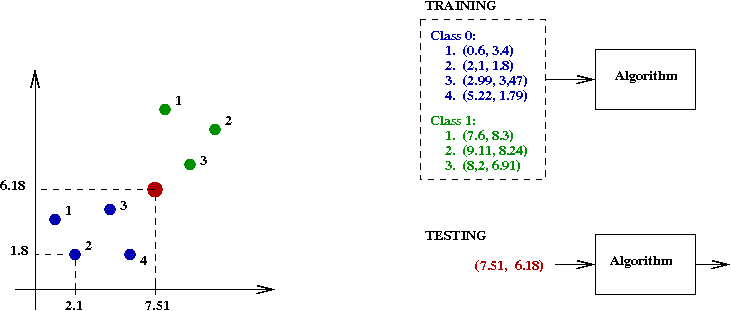
Exercise 7: For the point example (see the picture above) with $M=7$:
- What is $x^{(3)}$?
- What is $x_1^{(3)}$?
- What is $y^{(3)}$?
Thus, more formally, the training input to a problem is a collection of sample-label combinations:
$x^{(1)}$, $y^{(1)}$
$x^{(2)}$, $y^{(2)}$
$x^{(3)}$, $y^{(3)}$
...
$x^{(m)}$, $y^{(m)}$
where each $x^{(m)}$ is a sample and $y^{(m)}$ is the class the sample belongs to.
We will sometimes use the shorthand $y(x)$ to denote the true class (label) that $x$ belongs to.
$\Rightarrow$ $y^{(m)} = y(x^{(m)})$
Similarly, for testing data:
- We'll use $L$ to denote the number of test samples.
- In this case, the labels are not given to the algorithm.
  $\Rightarrow$ The algorithm is expected to provide the label.
- Thus the test data will be $d$-dimensional samples: $v^{(1)}, v^{(2)}, ..., v^{(L)}$
- In reality, there may be some "true answer" which may be known to the tester.
- As before, we'll use the notation $y(v)$ to denote the true (unknown) class for sample $v$.
Let $A$ denote an algorithm.
- During testing, $A(v^{(k)})$ denotes the response to the $k$-th test.
- Thus, ideally, $A(v^{(k)}) = y(v^{(k)})$.
  $\Rightarrow$ Otherwise, the algorithm makes a mistake.
A minor programming issue:
- Most of our notation is mathematical: e.g, $(x_1,x_2, ..., x_d)$.
  $\Rightarrow$ indexing starts with $1$.
- However, in our code, we'll start with $0$.
- Thus, we'll occasionally switch to $(x_0,x_2, ..., x_{d-1})$ where appropriate.

11.2 A simple learning algorithm: don't

We were only partly facetious:

The idea is this:

During training: merely store the training samples (i.e., don't learn).
During testing, use the stored data to try and classify test samples.

Thus, the training algorithm is trivial:

     Algorithm: nearestNeighborTraining (x^(m), y^(m))
     Input: M training samples x^(m), with labels y^(m)
     1.   Store x^(m), y^(m)

How to classify a test sample?
$\Rightarrow$ A simple idea: find the closest training sample and assign the class of that training sample.

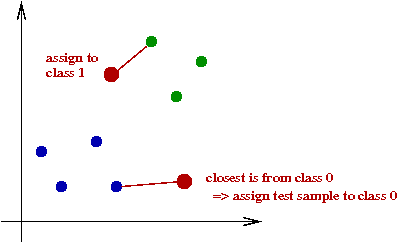
In pseudocode:

    Algorithm: nearestNeighborTest (v)
    Input: test sample v
    1.   best = 1
    2.   leastDistance = distance(x⁽¹⁾,v)
    3.   for m=2 to M
    4.       if distance(x^(m),v) < leastDistance
    5.           leastDistance = distance(x^(m),v)
    6.           best = m
    7.       endif
    8.   endfor
         // Return the class that training sample x^(best) belongs to.
    9.   return y(x^(best))

Exercise 8: Download (into the classifierJar directory) and modify NearestNeighbor.java to implement the Nearest-Neighbor algorithm.

Try it on the point problem for various numbers of generated points, and for different distributions.
Can you create a test point that makes it fail?
Apply the algorithm to the char problem. Why doesn't it work?

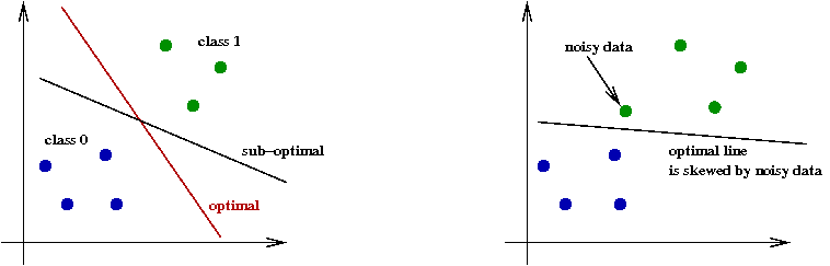
Improvements to Nearest-Neighbor:

Notice that a little noise in the data can easily result in poor classification:
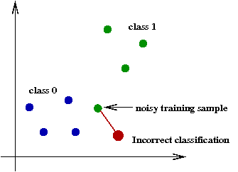
- A noisy sample near the boundary between two classes can wrongly favor the class of the noisy point.
- The noisy point stays in the training data
  $\Rightarrow$ The algorithm does not evaluate data quality.
K-Nearest-Neighbor:
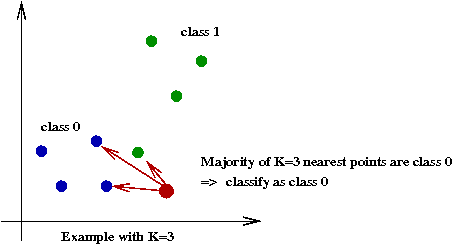
- Instead of relying on one point, try $K$
  $\Rightarrow$ Find the $K$ nearest points and pick the class most represented.
- Thus, the $K$ nearest points "vote" on the class to be assigned.
Exercise 9: What is the running time of K-Nearest-Neighbor in terms of $M$, the number of training samples, and $K$? Does $d$ matter in the running time? What data structure is most appropriate for this computation?

Exercise 10: Consider a database of $10^6$ greyscale images each of size 0.1 megabytes. For $K=10$, what is the number of arithmetic operations (say, multiplications) for a single classification? How would you calculate the distance between two images?
Thus, large data sets can slow down classification.
- This is particularly important when rapid classification is needed
  $\Rightarrow$ e.g., real-time applications such as handwriting recognition.
Second idea: pre-process the data to store fewer, but "representative" points:
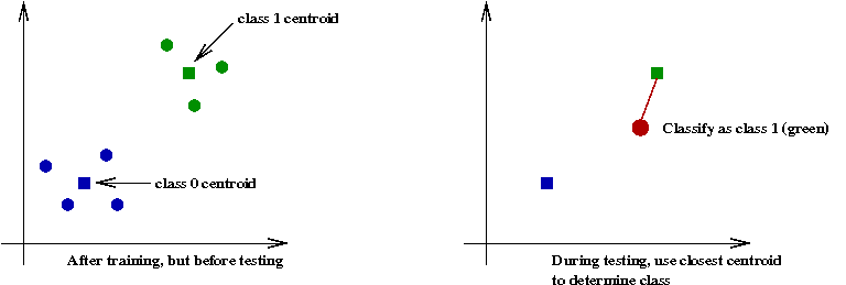
- In the most extreme version: store only the centroids of each class.
- However, the centroids can be skewed by noisy data.
- A variation: store a more representative sample.

Note: the idea of "condensing" the data into representative points is, in some sense, "learning"

     Algorithm: nearestNeighborTraining (x^(m), y^(m))
     Input: M training samples x^(m), with labels y^(m)
     1.   Preprocess into representative samples x'^(m), y'^(m)
     2.   Store x'^(m), y'^(m)

Third idea: use weighted distances:
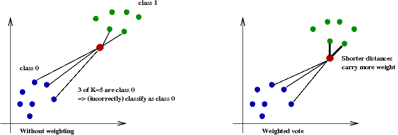
- Key idea: use the actual distance to the $K$ nearest neighbors.
- Let each neighbor's vote depend on this actual distance.
Fourth idea: use smarter data structures:
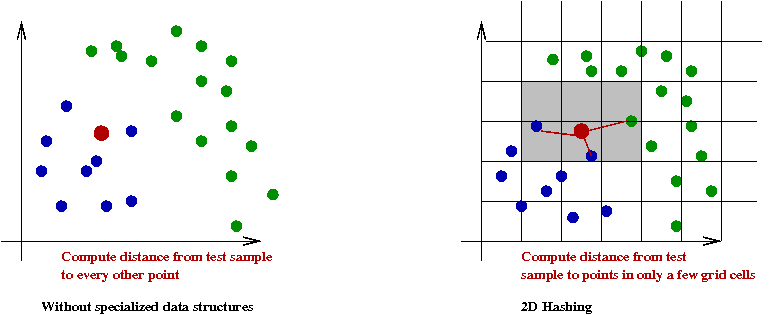
- Instead of performing distance calculations to each point
  $\Rightarrow$ Sharply reduce the number of distance calculations using a clever data structure.
- Example data structures: 2D hashtable, quadtrees, kd-trees.
- See Module 4 in CS-3212 for an explanation of 2D hashing.

Exercise 11: Download, compile and execute SimpleNN.java. You will also need DataGenerator.java.

Examine SimpleNN to confirm that it implements the Nearest-Neighbor algorithm for samples that come out of DataGenerator.
What is the probability of error?
Change the < to <= in the if condition at the end of classify(). What is the probability of error?
Explain why there's such a big difference.

11.3 A probabilistic viewpoint

Consider an example from the point problem:

Suppose our training data looked like this:

What rule could we use to classify future data points?

In this case, one might draw a line between the two "clouds":

$\Rightarrow$ In this case it's easy: there are many lines that appear to work.

However what if it turned out that future samples contradicted the clean separation?

To address this problem, we will consider the probability that a point came from class 0.

The probabilistic viewpoint, as we will see, results in two powerful concepts.

The first concept: the data can usefully be modeled as coming from distributions, even if we don't know the details of the distributions.

The second concept: using deciding-lines (or, in $d$ dimensions, hyperplanes) is the natural approach to try at first.

Before getting into the details, let's recall Bayes' rule:

In the "event" way of thinking, for any two events $A$ and $B$, $$ \prob{A | B} \eql \frac{\prob{B | A} \prob{A}}{\prob{B}} $$
In terms of rv's, for any two (discrete) rv's $X$ and $Y$, $$ \prob{X=k | Y=m} \eql \frac{\prob{Y=m | X=k} \prob{X=k}}{\prob{Y=m}} $$
Recall: it doesn't really matter whether one event "came before" (in the sense of causality or time).

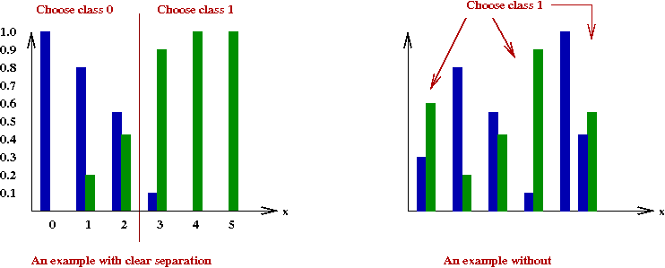
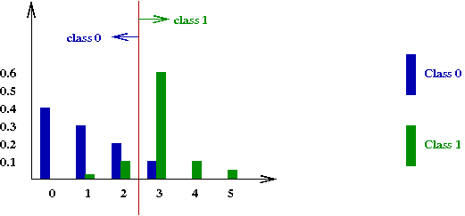
To simplify, we'll look at a discrete 1D example:

In this example, the data is taken from the set: $\{0,1,2,3,4,5\}$.
There are two classes: $c=0$ and $c=1$.

Exercise 12: Download DataExample.java and execute. You will also need DataGenerator.java and RandTool.java. Write code to estimate the probability that data is generated from class 0. What is the probability that the data comes from class 1?
Next, let's define some notation we'll need:
- Let rv $X$ denote the value (from $\{0,1,2,3,4,5\}$) produced in any one particular trial.
- Let rv $C$ denote the class.
- Note: you have just estimated $\prob{C=0}$ above.
Exercise 13: Add code to estimate $\prob{X=3 | C=0}$ and $\prob{X=3 | C=1}$.
- Why is it that the sum of these two does not equal 1? Which equation does result in 1?
- If you were given a test sample $x=3$ which of the two classes would you think it likely came from?
An examination of DataGenerator tells us how the data is generated:
- First, the generator chooses which class to generate from.
- Then, if class 0 is chosen, the output is generated according to some probabilities (in method generate0()).
- Likewise, if class 1 is chosen, the output is generated according to different probabilities (in generate1()).
We can write each of these down for class $0$:
$\prob{X=0 | C=0} = 0.4$.
$\prob{X=1 | C=0} = 0.3$.
$\prob{X=2 | C=0} = 0.2$.
$\prob{X=3 | C=0} = 0.1$.
$\prob{X=4 | C=0} = 0$.
$\prob{X=5 | C=0} = 0$.

Exercise 14: Write down the conditional pmf $\prob{X=m | C=1}$ by examining the code in DataGenerator.
Now consider two classification questions:
1. If the data happens to be $x=0$, which class did it likely come from?
  $\Rightarrow$ This is easy: it could only be class 0.
2. If the data happens to be $x=3$, which class did it likely come from?
Let's try this idea:
Given sample $x$, if $\prob{X=x|C=0} \gt \prob{X=x|C=1}$, classify $x$ as class $0$, else classify as class $1$.
Pictorially,
To evaluate this algorithm, we need a metric.
Let $\prob{E} = $ probability that the algorithm makes a mistake.

Exercise 15: Implement the algorithm in DataExample2.java, which has the code for evaluation. Try a different algorithm to see if the error improves.
Now let's consider an important point:
- We will limit our error to only those samples where $x=3$.
- Define $\prob{E_3} = $ probability that the algorithm makes a mistake when $x=3$.
Exercise 16: Copy the algorithm over to DataExample3.java, which estimates the error when $x=3$.
- What is the error?
- Next, change $\prob{C=0}$ (which is now 0.4) to 0.9. What is the error now?
- How would you change the algorithm to improve the error?
What we have seen is that the rule
If $\prob{X=x|C=0} \gt \prob{X=x|C=1}$, classify as class $0$, else classify as class $1$.
doesn't necessarily work.
Instead, consider the following rule:
Given $x$, if $\prob{C=0|X=x} \gt \prob{C=1|X=x}$, classify as class $0$, else classify as class $1$.
Unfortunately, we don't know $\prob{C=c|X=x}$.
$\Rightarrow$ We'll use Bayes' rule for this: $$ \prob{C=c|X=x} \eql \frac{\prob{X=x|C=c} \prob{C=c}}{\prob{X=x}} $$
Pictorially,
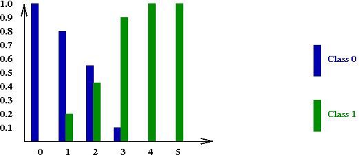
Thus, this new rule can be written as:
Given $x$, classify as class $0$ if $$ \frac{\prob{X=x|C=0} \prob{C=0}}{\prob{X=x}} \; \gt \; \frac{\prob{X=x|C=1} \prob{C=1}}{\prob{X=x}} $$
Since $\prob{X=x}$ cancels on both sides, the rule is:
Given $x$, classify as class $0$ if $$ \prob{X=x|C=0} \prob{C=0} \; \gt \; \prob{X=x|C=1} \prob{C=1} $$
$\Rightarrow$ This is called the Bayes' classification rule.

Exercise 17: For the case $x=3$, compute $\prob{X=x|C=0} \prob{C=0}$ and $\prob{X=x|C=1} \prob{C=1}$ by hand when $\prob{C=0}=0.4$. Then, compute both when $\prob{C=0}=0.9$.

Optimality of Bayes' classification rule:

Consider some algorithm A that differs from Bayes' rule.
If it differs, it must return the opposite class for some $x$.
Assume that for this particular $x$ it so happens that
$\prob{X=x|C=0} \prob{C=0} > \prob{X=x|C=1} \prob{C=1}$.
Thus, Bayes' chooses class 0.
$\Rightarrow$ Algorithm A chooses class 1.
Let's compute the error in this case: $$\eqb{ \probm{Bayes' makes an error} \eqt \prob{C=1|X=x} \;\;\;\;\;\;\;\;\;\;\;\;\;\;\;\;\;\;\;\;\; \mbox{(true class is 1 $\Rightarrow$ Bayes' makes a mistake)} \\ \eqt \frac{\prob{X=x|C=1} \prob{C=1}}{\prob{X=x}} \;\;\;\;\;\;\;\; \mbox{(simple application of Bayes' rule)} \\ & \; \lt \; & \frac{\prob{X=x|C=0} \prob{C=0}}{\prob{X=x}} \;\;\;\;\;\;\;\; \mbox{(this is how Bayes' algorithm works)} \\ \eqt \probm{A makes an error} }$$
Since the error can be summed across all the $x$ where the two algorithms differ, Bayes' is always superior.
$\Rightarrow$ The Bayes' classifier is optimal.
An important point: we did not assume that a single line separates the data:
The rule applies separately for each $x$.

The same idea applies to continuous distributions:

Suppose rv $X$ is continuous.
Let $f_0(x|C=0)$ be the conditional pdf of $X$ given the data comes from class $0$.
Similarly, let $f_1(x|C=1)$ be the conditional pdf of $X$ given the data comes from class $1$.
Then, the Bayes' classification algorithm is:
Given $x$, classify as class $0$ if $$ f_0(x|C=0) \prob{C=0} \; \gt \; f_1(x|C=1) \prob{C=1} $$

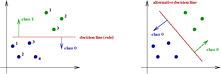
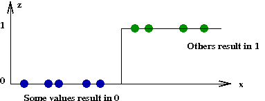
Let's now return to the idea of a separating line:

In 1D, since there is no line, we could call it a separating point:
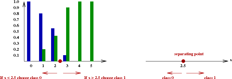
Here, there is some point $x_0$ such that our rule becomes:
Given $x$, choose class $0$ if $x \lt x_0$.
In 2D, this becomes a separating line:
How should our rule be written?
- Notice that our data points are now of the form: $x = (x_1, x_2)$.
- The equation of a line in 2D can be written in the form: $g(x) = 0$ where
  $g(x) = g(x_1,x_2) = w_1x_1 + w_2x_2 + w_3$.
In $d$ dimensions, we call this a separating hyperplane.
- Here, data points are of the form: $x = (x_1,x_2, ..., x_n)$.
- Fortunately, the equation for a hyperplane generalizes naturally from a 2D line: $g(x) = 0$ where
  $g(x) = g(x_1,x_2, ...,x_n) = w_1x_1 + w_2x_2 + ... + w_nx_n + w_{n+1}$.
Thus, the decision rule is this:
Given $x$, choose class $0$ if $g(x) \lt 0$. (Choose class $1$ otherwise).
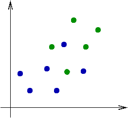
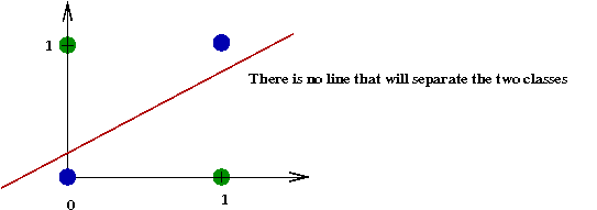
Does a separating line work for every problem?

Exercise 18: Give an example (with distributions) where it does not work.

A rationale for using separating hyperplanes:

Note that even if the given data is not separable, we could still use a line and allow for occasional errors:
Let's consider the 2D case when the conditional pdfs $f_c(x|C=c)$ are (2D) Gaussian.
In particular, when they are independent and have the same distribution.
What is a 2D Gaussian distribution?
- Here, each point is a rv $(X_1, X_2)$.
- Each $X_i$ is a Gaussian rv.
- Generating points from such a distribution results in a "cloud" of points.
One can show that the Bayes' rule is equivalent to a separating line when the variances are the same.
Unfortunately, if the variances are different, it turns out that the optimal separating curve is not a line.
$\Rightarrow$ Still, a line is a reasonable approximation if the variances are comparable.

What have we learned so far? Two important ideas:

Idea 1: There is some underlying distribution from which the data is drawn
$\Rightarrow$ We might need to study this distribution for more insight.
Idea 2: Using a separating hyperplane makes sense in many cases, and has a theoretical (Gaussian) foundation.

11.4 The best hyperplane

Let's now look at the problem of finding the best hyperplane for a given training set:

We will ignore the underlying distribution:

Even without knowledge of the distribution, one could discard outliers.
Knowledge of the distribution can help weight points, or discard others.
To gain knowledge about the distribution
$\Rightarrow$ Estimation problem.

Nonetheless, we'll proceed with finding the best hyperplane assuming the training points are representative.

We will need some notation:

We'll consider 2D first, for simplicity.
Let $w_1x_1 + w_2x_2 + w_3 = 0$ be the equation of the line.
For any point $(x_1,x_2)$, Let $A((x_1,x_2)$ denote the output of the algorithm.

What does "best" mean? First, let's understand how a "hyperplane" based algorithm works:

The basic idea is simple:

       if w₁x₁ + w₂x₂ + w₃ < 0
            classify as class 0
       else
            classify as class 1
       endif

Note: we could flip the classes around (in the if-statement).
$\Rightarrow$ It would only result in different constants (negating the constants).
Note: the "variables" to be optimized are: $w_1, w_2$ and $w_3$
$\Rightarrow$ They define the line.

Now, if we've found a line, let's ask how the algorithm performs against the training data:

Consider a training point $(x_1^{(m)},x_2^{(m)})$ and its true class $y^{(m)}$.
Let $\epsilon^{(m)} = (y^{(m)} - A(x_1^{(m)},x_2^{(m)}))^2$ be the error, the difference between true class and A's output.
Then the total error over all training samples $m$ is: $$ E \eql \sum_m \epsilon^{(m)} $$
Observe that $E$ is a function of $w_1, w_2, w_3$ because each $\epsilon^{(m)}$ depends on these $w_i$'s.

Thus, to minimize $E$, one can evaluate $E$ over various choices of the $w_i$'s.

Unfortunately, this is impractical for two reasons:

For realistic problems, the dimension is too large
$\Rightarrow$ Something like bracket-search would collapse when $d=100$ (char example).
$E$ is not a differentiable function of the $w_i$'s.

Exercise 19: Why isn't $E$ differentiable with respect to $w_i$?

Instead we will opt for a simple approximation:

Consider a point $(x_1,x_2)$.
If $y(x_1,x_2) = 1$, but $A(x_1,x_2) = 0$, the algorithm makes an error.
Notice that $w_1x_1 + w_2x_2 + w_3 \lt 0$ in this case.
Thus, a better choice of $w_i$'s will result in $w_1x_1 + w_2x_2 + w_3 \gt 0$.
This choice will lessen the distance $$ y(x_1,x_2) \; - \; w_1x_1 - w_2x_2 - w_3 $$
A symmetrically equivalent reasoning applies to the case when If $y(x_1,x_2) = 0$, but $A(x_1,x_2) = 1$,
- Here, once again, we want to lower the distance between $w_1x_1 - w_2x_2 - w_3$ and $y(x_1,x_2)$.
Now, for any training sample, $(x_1^{(m)},x_2^{(m)})$ let $$ \epsilon^{(m)} \eql (y^{(m)} - w_1x_1^{(m)} - w_2x_2^{(m)} - w_3)^2 $$
Note: $\epsilon^{(m)}$ is a function of the $w_i$'s.
The intuition: minimizing the squared error should lower the "distance" we seek to minimize when the algorithm is "wrong".
For brevity, define $$ S^{(m)} \eql w_1x_1^{(m)} + w_2x_2^{(m)} + w_3 $$
Then, $$ \epsilon^{(m)} \eql (y^{(m)} - S^{(m)}) $$
Define the approximate error $$ E(w_1,w_2,w_3) \eql \sum_m \epsilon^{(m)} $$
Note: $E$ is a function of the $w_i$'s.
In fact, even better, $E$ is a differentiable function of the $w_i$'s.

Exercise 20: Why?

Let's use gradient descent:

First, since is a multivariable problem, we will need to compute partial derivatives.
- Let $$\eqb{ \epsilon_i^{(m)} \eqt \frac{\partial \epsilon^{(m)}}{\partial w_i} \eqt \mbox{partial derivative of $\epsilon^{(m)}$ with respect to $w_i$} }$$
- Since $$ \epsilon^{(m)} \eql ( y^{(m)} - w_1x_1^{(m)} - w_2x_2^{(m)} - w_3 )^2 $$ the partial derivative with respect to $w_i$ is $$\eqb{ \epsilon_i^{(m)} \eqt \frac{\partial}{\partial w_i} (y^{(m)} - w_1x_1^{(m)} - w_2x_2^{(m)}- w_3 )^2 \\ \eqt - 2 (y^{(m)} - w_1x_1^{(m)} - w_2x_2^{(m)} - w_3) x_i\\ \eqt - 2 (y^{(m)} - S^{(m)}) x_i }$$
- Next, let $E_i'$ denote the partial derivative of $E$ with respect to $w_i$. Then, $$\eqb{ E_i' \eqt \frac{\partial}{\partial w_i} \sum_m \epsilon^{(m)}\\ \eqt \sum_m \epsilon_i^{(m)} }$$
- For gradient descent, we need $E_i'$ to update each $w_i$.

Then, gradient descent can be applied to each variable:

     Algorithm: computeOptimalWeights (x^(m), y^(m))
     Input: M training samples x^(m), y^(m)
     1.    Initialize w_i's.                   // Most often: to some small non-zero values.
     2.    while not converged
     3.        for each i
     4.            E_i' = 0
     5.            for each m
     6.                compute partial derivative ε_i^(m)
     7.                E_i'= E_i' + ε_i^(m)
     8.            endfor
     9.        endfor
     10.       for each i
     11.           w_i = w_i - α E_i'
     12.       endfor
     13.   endwhile
     14.   return w_i's.

We're now in a position to describe both training and testing for this approach:

Training:

     Algorithm: gradientTraining (x^(m), y^(m))
     Input: M training samples x^(m), y^(m)
     1.    computeOptimalWeights (x^(m), y^(m))
     2.    store weights

Testing:

     Algorithm: gradientClassification (x)
     Input: test sample x = (x₁, ..., x_d)
     1.    S = w₁x₁ + ... + w_dx_d + w_d+1
     2.    if S < 0
     3.        return 0          // Classify as class 0
     4.    else
     5.        return 1          // Classify as class 1
     6.    endif

Lastly, a small point about convention:
- It is sometimes convenient to use "-1 and 1" instead of "0 and 1" for the two classes.

Exercise 21: Download Gradient.java into your classiferJar directory.

Examine the code and verify that gradient descent (with line-search) is being used.
Use this algorithm as the classifier to classify 100 points in the point problem.
Add code to plot the separating line in a Function object.
Reduce the number of iterations to 500. What is the result?
How does the algorithm perform without line-search?

A further approximation:

Notice that we sum over all samples $m$ in computing the partial derivative $E_i'$.
This approach has two disadvantages:
- If $m$ is large, it's a large calculation.
- It cannot be used for incremental training
  $\Rightarrow$ when you want to intersperse testing with training.
Exercise 22: In what application would we want to intersperse testing with training?
Suppose we want to update the weights $w_i$ after each training sample.

As an approximation, we could leave out the other $m$'s

     while not converged
         for each m
             compute partial derivative ε_i^(m)
             for each i
                 w_i = w_i - α E_i'
             endfor
         endfor
         // Note: the weights may be used here for testing.
     endwhile

This approximation is called the Widrow-Hoff rule, or sometimes, the Delta-rule.

A few more comments:

The $w_i$'s are often called weights.
Given a test sample, the algorithm checks whether $w_1x_1 + w_2x_2 + w_3 \gt 0$,
$\Rightarrow$ Equivalent to seeing whether $w_1x_1 + w_2x_2 \gt - w_3$,
This is of the form
Check whether weighted sum of $x_i$'s is greater than a threshold (that happens to be $-w_3$).
Thus, we sometimes refer to the training as "training the weights".
The $w_i$'s are algorithm parameters.

11.5 Minimizing an alternative error function: the perceptron

The perceptron is a simple and historically pivotal algorithm:

The perceptron is only slightly different than the Delta rule, as we'll see, but simpler.

First, for a given set of weights and given input, a perceptron applies the same weighted-sum as before:

     Algorithm: applyPerceptron (x)
     Input: a sample x
           // Apply the current weights and check against threshold.
     1.    S = w₁x₁ + ... + w_dx_d + w_d+1
     2.    if S > 0
     3.        return 1
     4.    else
     5.        return 0
     6.    endif

Training:

     Algorithm: perceptronTraining (x^(m), y^(m))
     Input: M training samples x^(m), y^(m)
     1.    Initialize w_i's.                   // Most often: to some small non-zero values.
     2.    while not converged
     3.        for each m
     4.            z^(m) = applyPerceptron (x^(m))
     5.            for each i
     6.                w_i = w_i + α (y^(m) - z^(m)) x_i^(m)
     7.            endfor
     8.        endfor
     9.    endwhile
     10.   return w_i's.

Testing: this is the same as applying the perceptron.

Intuition:

Consider a sample where $y^{(m)} = 1$, but the predicted class is $z^{(m)} = 0$.
Then, the update
$w_i = w_i + \alpha (y^{(m)} - z^{(m)}) x_i^{(m)}$
has the effect of increasing the weights.
This is exactly what we want because larger weights increase the possibility that the weighted sum will exceed the threshold.
Similarly, when the weighted sum is too large, we want to decrease the weights.

The perceptron algorithm is really gradient descent applied to a different objective function:

Define the error $E = \sum_m (y^{(m)} - z^{(m)})$.
$\Rightarrow$ This is not the mean-squared error we used for the Delta rule.
We will distinguish between the two cases when the algorithm makes a mistake:
- Let M' = set of samples such that $y^{(m)} = 1$ but $z^{(m)} = 0$
- Let M'' = set of samples such that $y^{(m)} = 0$ but $z^{(m)} = 1$
Accordingly, we will break the error into two parts:
1. $E' = \sum_{m\in _M'} (y^{(m)} - z^{(m)})$.
2. $E'' = \sum_{m\in M''} (y^{(m)} - z^{(m)})$.
Then, notice that we want to minimize $E'$ and maximize $E''$ (because of the sign).
This is the same as minimizing $E' - E''$.
Next, observe that $E$ is not differentiable with respect to $w_i$ (because $z$ is a step-function).
Once again, we'll approximate the error by using the direct (un-stepped) difference
$E = \sum_m (y^{(m)} - w_{d+1} - \sum_i w_i x_i) $
Similarly, we'll take $E'$ and $E''$ to represent the un-thresholded difference.
In this case, the derivative of $E'$ with respect to $w_i$ is simply $-x_i$ (the coefficient of $w_ix_i$).
Likewise, the derivative of $E''$ with respect to $w_i$ is $x_i$.

Thus, gradient descent would look like:

       if m ε M'
           w_i = w_i - α (- x_i)   
       else
           w_i = w_i - α (x_i)

But this is exactly what the algorithm does, by using $(y^{(m)} - z^{(m)})$ as the sign.

More about perceptrons:

One can show that if a training set is actually linearly separable, there is a small enough stepsize that'll get the perceptron to converge to an acceptable hyperplane.
Two-input perceptrons can be used to emulate some logic: AND, OR, NAND functions for example.
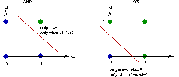
However, perceptrons cannot handle data that is not linearly separable, such as the XOR function:

11.6 Addressing the differentiability problem

Recall that the true error function was not differentiable:

With the gradient algorithm or the Delta rule, we instead differentiated an approximate error.
$\Rightarrow$ By ignoring the step function

Another approach: use a differentiable function.

What we would like:

Given input $x = (x_1, ..., x_d)$, and algorithm parameters $w = (w_1, w_1, ... )$ compute $z = f(x, w)$.
Then use $z$ to decide which class.
Ideally, we want $f$ to be differentiable with respect to $w_i$.
Ideally, we'd also like to use hyperplanes.

Consider a single dimension $d=1$:

Earlier, we used the rule:

         if z < 0
             classify as class 0
         else
             classify as class 1.
         endif

Thus, the output values $z$ are either 0 or 1 for any $x$:

Suppose instead we used the following:

        z = f(x, w)
        if z is closer to 0
            classify as class 0
        else
            classify as class 1
        endif

Here, we will strive to make $f$ a differentiable function.
Ideally, we want a differentiable function that will be as close to the "ideal" step function above, yet differentiable.

One such popular function: the sigmoid function $$ f(s) \eql \frac{1}{(1 + e^{-s})} $$

Exercise 23: Download and add code to Sigmoid.java to compute and display the sigmoid function in the range [-10,10]. You will also need Function.java and SimplePlotPanel.java How could you make it approximate a step function even more closely?

Exercise 24: Show that the sigmoid derivative is $f'(s) = f(s) (1 - f(s))$.

How is the sigmoid used?

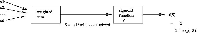
Define $S = w_1x_1 + ... + w_dx_d + w_{d+1}$ to be the weighted sum (including threshold).
To compute the output, simply compute $f(S)$ and round.
During training, use the derivatives: $$\eqb{ \frac{\partial z}{\partial w_i} \eqt \frac{\partial f(S)}{\partial w_i}\\ \eqt f(S) (1 - f(S)) \frac{\partial S}{\partial w_i} }$$
- We have already computed $\frac{\partial S}{\partial w_i}$
  $\Rightarrow$ This is what we used in the gradient algorithm.

11.7 Neural networks

Recall the difficulty with XOR:

A single line cannot separate the 1's from the 0's in XOR.

However, we could combine multiple lines:

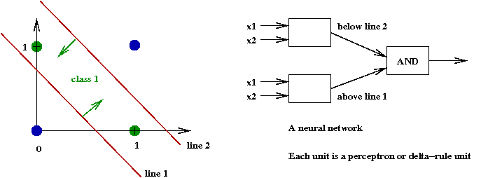
Exercise 25: Determine weights for each of the three units above so that the result achieves the XOR function. Then, build a truth table and show how the combination results in computing XOR.

By treating the earlier algorithms (perceptron, delta-rule) as a single unit, we can build networks of such units:

The hope is that we can learn more complex input-output functions that can classify a given data set.

The two-layer backpropagation algorithm:

We will now examine a simple, and popular two-layer algorithm called backpropagation.
There are two ideas at work here:
- Each unit will use sigmoids, allowing for differentiable error functions.
- The error function will be the mean-square.
- We will use an approximate gradient descent to create an iterative algorithm
  $\Rightarrow$ This algorithm will be applied to the training set samples.
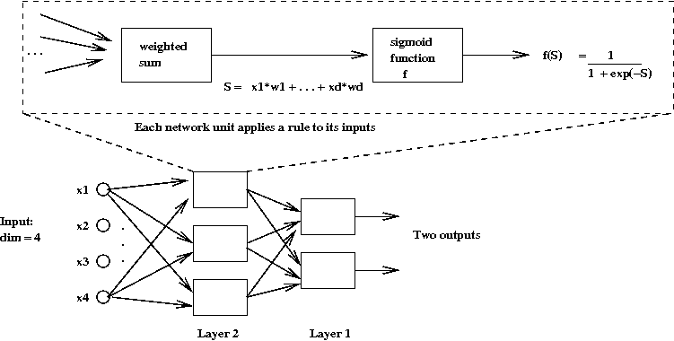
The network structure has two layers:
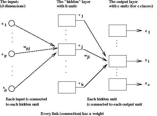
- The first layer is the so-called hidden layer.
- Each input $x_i$ is fed into each hidden unit.
  $\Rightarrow$ Each hidden unit must have $d+1$ weights.
- Let $v_j$ denote the output value of the $j$-th hidden unit. (Here, $(j=1, ...,h)$.)
- The output of each hidden unit is connected to each of the $c$ output units.
  $\Rightarrow$ Each output unit must have $h+1$ weights.
- Thus, it's natural to associate the weights with the connections.
The $j$-th hidden unit computes $$ v_j \eql f(\sum_p w_{pj} x_p) $$ where $f$ is the sigmoid function.
Similarly, the $i$-th output unit computes $$ z_i \eql f(\sum_j w_{ji} v_j) $$ because the $v_j$'s are the inputs to those units.

Next, let us understand how the network is applied to a particular test sample:

     Algorithm: applyBackPropagation (x)
     Input: a sample x
           // Compute the outputs of the hidden units
     1.    for each hidden unit j
     2.        S_j = w_1jx₁ + ... + w_djx_d + w_d+1,j
     3.        v_j = f(S_j)
     4.    endfor
           // Now compute the outputs of the output units
     5.    for each output unit i
     6.        S_i = w_1iv₁ + ... + w_hiv_h + w_h+1,i
     7.        z_i = f(S_i)
     8.    endfor
     9.    Find the largest z_i among z₁, ..., z_c
           // Classify into class i.
     10.   return i

For the training part, we will apply the gradient descent principle:

Define $z^{(m)}$ as the final output for the $m$-th training sample.
Define the error $$ E \eql \frac{1}{2} \sum_m (y^{(m)} - z^{(m)})^2 $$
First, we will compute partial derivatives with respect to the weights in the output layer: $$\eqb{ \frac{\partial E}{\partial w_{ji}} \eqt - (y_i - z_i) \frac{\partial z_i}{\partial w_{ji}} \\ \eqt - (y_i - z_i) \frac{\partial f(S_i)}{\partial S_i} \frac{\partial S_i}{\partial w_{ji}} \\ \eqt - (y_i - z_i) f(S_i)(1 - f(S_i)) \frac{\partial S_i}{\partial w_{ji}} \\ \eqt - (y_i - z_i) f(S_i)(1 - f(S_i)) v_j }$$
Thus, the update rule for these weights will be $$ w_{ji} \eql w_{ji} + \alpha (y_i - z_i) f(S_i) (1 - f(S_i)) v_j $$ where $y_i$ = i-th component of $y^{(m)}$ and $z_i$ = i-th component of $z^{(m)}$.
For the hidden layer units, there's an additional step because the output $z_i$ depends on all the hidden layer weights.
- First, apply the chain rule: $$ \frac{\partial E}{\partial w_{pj}} \eql \frac{\partial E}{\partial v_j} \frac{\partial f}{\partial S_j} \frac{\partial S_j}{\partial w_{pj}} $$
- Then, observe that $$ \frac{\partial f}{\partial S_j} \eql f(S_j) (1 - f(S_j)) $$ and $$ \frac{\partial S_j}{\partial w_{pj}} \eql x_j $$
- Lastly, $$\eqb{ \frac{\partial E}{\partial v_j} \eqt - \sum_i (y_i - z_i) \frac{\partial z_i}{\partial v_j}\\ \eqt - \sum_i (y_i - z_i) \frac{\partial f(S_i)}{\partial S_i} \frac{\partial S_i}{\partial v_j} \\ \eqt - \sum_i (y_i - z_i) f(S_i) (1 - f(S_i)) w_{ji} }$$
- Putting these together, we get $$ \frac{\partial E}{\partial w_{pj}} \eql - x_j f(S_j) (1 - f(S_j)) \sum_i (y_i - z_i) f(S_i) (1 - f(S_i)) w_{ji} $$
Thus, the update rule for the hidden layer is: $$\eqb{ w_{pj} \eqt w_{pj} + \alpha \frac{\partial E}{\partial w_{pj}}\\ \eqt w_{pj} + \alpha x_j f(S_j) (1 - f(S_j)) \sum_i (y_i - z_i) f(S_i) (1 - f(S_i)) w_{ji} }$$ Note: we've absorbed the minus sign into the constant $\alpha$.
Whew!

Finally, the training algorithm can be written as:

     Algorithm: backpropagationTraining (x^(m), y^(m))
     Input: M training samples x^(m), y^(m)
     1.    Initialize weights w_ji's and w_pj's
     2.    while not converged
     3.        for each m
     4.            z^(m) = applyBackpropagation (x^(m))
                   // Change the weights of the hidden layer:
     5.            for each w_pj
     6.                w_pj = w_pj + α x_j f(S_j)(1 - f(S_j)) Σ_i (y_i - z_i) f(S_i) (1 - f(S_i)) w_ji.
     7.            endfor
                   // Change the weights of the output layer:
     8.            for each w_ji
     9.                w_ji = w_ji + α (y_i - z_i) f(S_i) (1 - f(S_i)) v_j
     10.           endfor
     11.       endfor
     12.   endwhile

11.8 Feature extraction

Consider the following simple example:

Suppose we have the following data ($d=10$) for two classes:

    class 0:
       m=1:   1 0 1 1 1 0 1 0 0 0 
       m=2:   0 0 1 0 1 1 0 0 0 1 
       m=3:   1 0 1 1 1 1 0 1 0 0 

    class 1:
       m=1:   0 0 0 1 0 0 1 1 1 1 
       m=2:   0 0 0 1 0 0 1 1 1 1 
       m=3:   1 0 0 0 1 1 0 1 0 1

Here, each $x_i^{(m)}$ happens to be binary.

Notice that $d=10$.

Next, observe $x_3$ in the data:

    class 0:
       m=1:   1 0 1 1 1 0 1 0 0 0 
       m=2:   0 0 1 0 1 1 0 0 0 1 
       m=3:   1 0 1 1 1 1 0 1 0 0 

    class 1:
       m=1:   0 0 0 1 0 0 1 1 1 1 
       m=2:   0 0 0 1 0 0 1 1 1 1 
       m=3:   1 0 0 0 1 1 0 1 0 1

$\Rightarrow$ Obviously, $x_3$ alone differentiates the two classes.

Thus one aspect of feature extraction is to extract key elements of the data to help a classification algorithm.
$\Rightarrow$ This is done prior to training.

Consider this example:

    class 0:
       m=1:   1 0 1 1 1 0 1 0 0 0 
       m=2:   0 1 1 0 1 1 0 0 0 1 
       m=3:   1 0 1 1 1 1 0 1 0 0 

    class 1:
       m=1:   0 0 0 1 0 0 1 1 1 1 
       m=2:   0 0 0 1 0 0 1 1 1 1 
       m=3:   1 0 1 0 1 1 1 1 0 1

In this case, no single column distinguishes the two classes.

However, suppose we count the number of 1's in each half of each sample, e.g.,

              1 0 1 1 1 0 1 0 0 0     // First half has 4 one's.
              1 0 1 1 1 0 1 0 0 0     // Second half has 1 one.

This gives us two numbers (4,1) for each sample.

Let's do this for each sample:

    class 0:
       m=1:   1 0 1 1 1 0 1 0 0 0    → (4, 1)
       m=2:   0 1 1 0 1 1 0 0 0 1    → (3, 2)
       m=3:   1 0 1 1 1 1 0 1 0 0    → (4, 2)

    class 1:
       m=1:   0 0 0 1 0 0 1 1 1 1    → (1, 4)
       m=2:   0 0 0 1 0 0 1 1 1 1    → (1, 4)
       m=3:   1 0 1 0 1 1 1 1 0 1    → (3, 4)

Thus, class 0 samples have more 1's in the first half than in the second.
$\Rightarrow$ The opposite is true for class 1.

Thus, the training samples given to the algorithm could simply be:

    class 0:
       m=1: (4, 1)
       m=2: (3, 2)
       m=3: (4, 2)
    class 1:
       m=1: (1, 4)
       m=2: (1, 4)
       m=3: (3, 4)

Note: the same feature extraction that is applied to training samples must be applied to test samples:

Suppose we want to classify

             0 0 1 0 0 0 1 0 1 1

We'd convert this to (1,3)

             0 0 1 0 0 0 1 0 1 1    → (1, 3)

Here, the dimension of the reduced sample is $d=2$.

This second example is perhaps more important:

For large dimensions, it helps to look at the distribution of values in a single sample.
These distributions can become the features that are fed as training samples to an algorithm.

Exercise 26: Consider the point problem from earlier. Can any dimensions be ignored for this problem?

Let's consider some ideas for the char problem:

Recall: a single char is a collection of (tiny) line segments.
The first idea is to examine the distribution of these segments in 2D space:
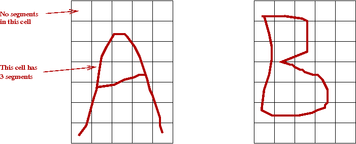
- We lay a fixed-size (M x N) grid over each char.
- For each cell, count the number of segments that intersect with that cell.
  $\Rightarrow$ This will give us a training sample of size $MN$.
- For example (for "A" above):
```
       0 0 0 0 0     // M=7 rows, N=5 columns
       0 1 2 0 0
       0 2 1 3 0
       0 3 2 4 0
       0 4 1 2 0
       2 1 0 0 2
       2 0 0 0 2
       
```
- When converted into a training sample of dimension $d = M x N$ = 35.
```
       0 0 0 0 0   0 1 2 0 0  0 2 1 3 0  0 3 2 4 0  0 4 1 2 0  2 1 0 0 2  2 0 0 0 2
       
```
  (We have inserted spaces for readability).
The second idea: examine the distribution of segment angles:
- Suppose we have an "A" with 5 segments:
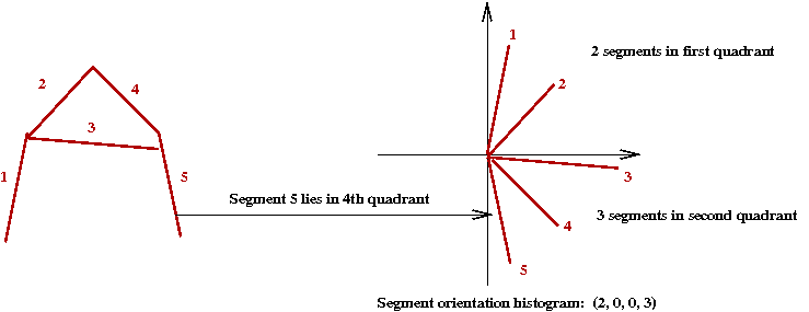
- Similarly, for a "B" with 7 segments:
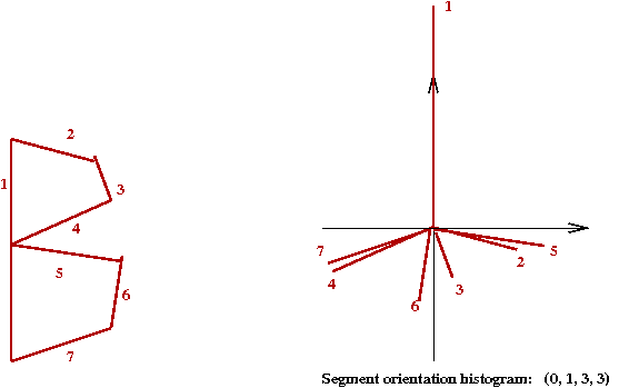
Two other refinements to this second idea:
- Notice that the (angle) histogram has 4 bins
  $\Rightarrow$ In practice, a larger number (10) is probably more useful.
- Because the actual orientation of the char may vary
  $\Rightarrow$ It helps to order the histogram by starting with the largest bin.
We have only scratched the surface of feature extraction for handwritten text
$\Rightarrow$ For full text, and placement within a page, there are far more issues that must be considered.
For example, see this project about address recognition from postal envelopes.

What about our third problem - face recognition?

Clearly, feature extraction is highly domain-specific
$\Rightarrow$ Detailed knowledge of the application and the data type is useful.
What kinds of information can we extract from images?
$\Rightarrow$ Obvious properties include: intensity, color, size.
But do these properties really help?
$\Rightarrow$ Sometimes a histogram of intensities or color can make a difference.
We will, however, consider a different approach - one that is similar to the segment-orientation idea for chars.
Step 1: convert to greyscale.
Next, recall that a greyscale image is just a 2D array of intensities.
Step 2: define a collection of (possibly overlapping) blocks to cover the image:
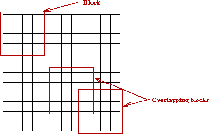
Step 3: For each block, compute a histogram of gradient orientations:
- You are thinking ... where are the gradients in an image?
- We will compute a gradient orientation at each pixel (in a block).
  $\Rightarrow$ The histogram is merely the histogram of these values.
- So what is the gradient orientation at a pixel? Let $A[i,j]$ denote the pixel at row $i$, column $j$.
- First, compute the average change in $x$ and $y$ directions separately:
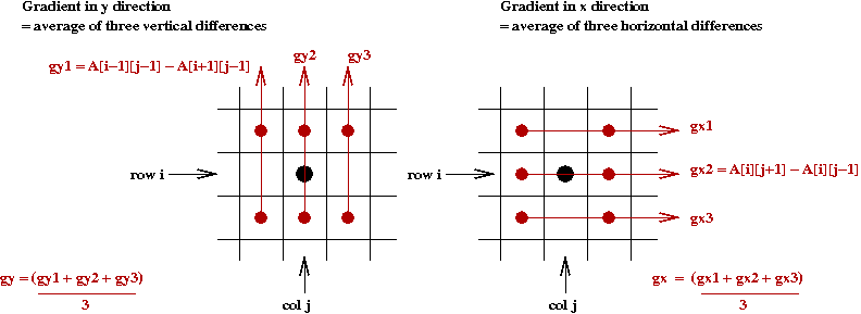
- Then consider the values $(g_x, g_y)$.
  $\Rightarrow$ The orientation (angle) is $a_{i,j} = \tan^{-1} (g_y / g_x)$
- A histogram of $a_{i,j}$ values is computed for each block (using some bin size).
- These histograms are then concatenated together into a large vector
  $\Rightarrow$ This vector becomes the training sample.
Additional detail about this technique can be found in this Wikipedia article.

Exercise 27: Examine the file FaceFeatures.java in the classifierJar directory to confirm that this method is implemented by the class FaceFeatures2. Switch to using this class, and try to classify test images using NearestNeighbor.

11.9 Summary

What have we learned in machine learning?

We've seen that feature extraction and learning can be separated:

Feature extraction is domain-specific.
$\Rightarrow$ One needs to custom-design a feature extractor for each type of problem.
The learning algorithms can be quite general.

We focused in particular on the classification problem.

The key ideas came from applying probability and optimization
$\Rightarrow$ In particular, conditional distributions and gradient descent.

What else is there to learn in machine learning?

We have only scratched the surface (a few textbook chapters) of machine learning.
There are various specialty areas with algorithms:
- Support vector machines.
- Logistic regression.
- Decision trees.
- Inductive learning.
Techniques for improving the training process:
- Boosting (how to make any algorithm better).
- Careful pre-processing of samples to pick more representative ones, and remove outliers.
There are also a variety of problem types:
- Unsupervised learning (when labels are not known).
- Temporal learning (learning over a sequence of steps).
- State-based learning (hidden markov models).
The deep and growing connection with statistics:
- We've seen that classification is really a type of prediction.
- In statistics, the problem is often called regression.
The applications are many and growing. Examples of successful ones:
- Speech, face, handwriting recognition.
- Gene finding (bioinformatics).
- Bio-sample classification.
- Natural language parsing.
- Text understanding.
- Security (biometrics).