In-Class Exercise 1:
Download, compile and execute Arm.java.
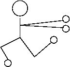
You will see a robotic arm and a circular (green) target hidden
behind some (red) obstacles.
You can click on a (blue) joint and move it.
Goal: move the arm so that the tip of the arm touches the target
without touching the obstacles, and while remaining entirely
within the drawing space.
In-Class Exercise 2:
Download carSim.jar,
unpack and execute CarGUI by typing java CarGUI manual
at the command-line.
- In Scene-1, use each of the three non-accelerative
cars (unicycle, simple-car, Dubin-car) to reach the target.
After clicking "reset" and then "go",
apply the slider controls (C1, C2) to move the car.
Each time you use a car,
you'll need to click "Reset" after setting the parameters.
- Repeat the same for the accelerative version of the Unicycle.
What is the difference in the time taken?
- Try a few more cases: (1)
In Scene-3, use the Dubin car to reach the target.
(2) In Scene-4, use the Simple car.
In-Class Exercise 3:
Next, write your own controller:
- Implement code in the move() method
of SimpleCarController to set the velocity
and steering angle.
- To see your controller in action, type java CarGUI
auto at the command-line, then load your controller
by typing SimpleCarController
in the textbox next to the "load controller" button, then
clicking on the button.
After this, click "reset" and then "go".
- What happens when you keep the steering angle constant?
- Can you write controls to get to the target in Scene-3?
In-Class Exercise 4:
How would one define a robot?
Is a coffee-maker a robot? A vending machine?
In-Class Exercise 5:
Identify some creative and possibly futuristic applications
of robots. Write down a list of computer-science challenges
to be addressed in developing such applications.
Write down examples of robotics problems that you
consider "easy" or "solved".
0.2 Second of three problems: Simulation
We actually did see an example of simulation already:
the physical modeling and simulation of car movement.
Next, consider a simple inventory system:
- A store has a single product and a single warehouse
with capacity C.
- Customers arrive at random (unknown) moments and
purchase items.
- When the stock gets too low (lower than threshold M),
we order an amount A from the supplier.
- There are two kinds of costs: (1) "lost" customers
(customers who arrive to find the warehouse empty);
(2) "holding" cost - each item held for a unit of time
in the warehouse costs money.
In-Class Exercise 6:
Identify (qualitatively) the tradeoffs between lost-customers and
holding costs:
- What happens as M increases or decreases
for fixed A?
- What happens as A increases or decreases
for fixed M?
In-Class Exercise 7:
Download Inventory.java,
UniformRandom.java
and stick.png. Then compile and
execute Inventory.java. Try
these values (click "reset" for each):
- C=10, M=3, A=6
- C=10, M=3, A=2
- C=10, M=3, A=3
What do you observe?
In-Class Exercise 8:
There is a very essential difference between the type
of simulation in the car-control example and type of
simulation in the inventory example.
Can you identify this difference (or differences)?
Are there similarities?
0.3 Third of three problems: Machine Learning
In-Class Exercise 9:
Download and execute PointClassifier.java.
Enter the following data:
- "Red" points: (50,250), (100,200), (125,225), (125,250), (125,325).
- "Blue" points: (200,125), (225,225), (250,75), (275,175), (300,100).
Clearly, it's easy to tell the groups apart. Next, use another color
to enter these points:
- Enter (75,225). Is is easy to tell whether this belongs to the
"red" vs. "blue" group?
- What about (500,150) or (500,400)?
- What about (150,160)?
In-Class Exercise 10:
Modify the above program
(PointClassifier.java)
to draw a line that best separates the two clusters of points.
Implement your code in the paintComponent() method.
In-Class Exercise 11:
One way to classify a new point is to see which side of
a dividing-line (like the one you drew above) the point
lies. Suggest one or more metrics to quantify the usefulness
of a particular line (so that we could compare alternative lines).
In-Class Exercise 12:
Download and unpack classifier.zip.
There are three sets of data files. One set, the "A" set has
all the file names beginning with "A". The "B" set has five
beginning with "B". And there is one "sample".
- Examine one of the "A" files. You will see that it is
a collection of line segments. Each data file defines
a collection of line segments.
- Every "A" file is similar in some way to every other "A" file.
- Every "B" file is similar in some way to every other "B" file.
- The big question: is the "sample" file more similar to an "A"
type or a "B" type?
- To answer the question, modify the code in
Classifier.java to print some statistic related to each collection.
To do this, you can simply insert code into the
printData() method.
- Note that each line segment is available to you as an instance
of LineSegmentd.
- Follow instructions in class to "view" the data files.
In-Class Exercise 13:
How are the two classification problems related?
Have you interacted with a system using classification?
Can you list some examples?
0.4 What do the three problems have in common?
Many things:
- All three are areas of growing importance in computer science.
- Underlying all three are key algorithmic questions:
- How do you devise algorithms for robot control?
- How do you write a simulation?
- How do you devise algorithms for classification and learning?
- None of these algorithms are covered in a standard algorithms course.
- The type of mathematics behind these areas is mostly continuous
=> As opposed to the discrete mathematics in the
standard algorithms course.
To better understand this distinction, let's start with
discrete structures:
In-Class Exercise 15:
Find an undergraduate math curriculum and classify courses
into "discrete" and "continuous".
0.5 What this course is about: The Other Side of Algorithms
Main goal: to study algorithms based on continuous structures.
Specifically:
- Algorithms for computing with real numbers.
- Computational view of key concepts in
continuous mathematics: limits, continuity, calculus.
- Algorithms for simulating systems with
deterministic continuous variables.
- Computational view of key concepts in
probability.
- Algorithms for simulating systems with
probabilistic components.
- Algorithms for continuous optimization problems.
- Application areas:
- Robotics: simulation and control.
- Simulation: computational modeling, simulation of physical
systems (molecules, highway traffic, space travel)
- Machine learning: classification, learning and adaptation.
- Other topics, time permitting:
statistical NLP, reinforcement learning.