- Write a simulator and GUI for this problem. Your GUI should have "Go" and "Quit" buttons, should depict the two cars going across from left to right and should show the point the two cars meet. Your simulator should find the distance traveled for each car as a function of time.
- At what time and distance does the trooper catch up with the speeding car?
- What is the trooper's speed at the moment they catch up?
a(t) = g - k v(t)
where k is a constant that depends on the air-resistance offered by the skydiver. Suppose the skydiver pops the chute at time t=T. Then, we will assume k=0.268 (low drag) when t<T (before the chute opens) and k=1.342 (high drag) after the chute opens.
- Write a simulator for this problem and a simple GUI depicting the skydiver - make sure that something changes on screen to differentiate between freefall and when the chute is open. Your GUI should have a "Go" button and a "Quit" button. You can, of course, make your GUI elaborate (use an image of a skydiver etc).
- Suppose that the skydiver is able to land at a velocity of 40 feet/sec. When should the chute be opened at the latest assuming the fall starts at a height of 1200 feet?
- Plot the velocity function for the skydiver.
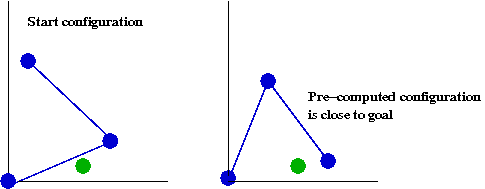
In the picture above, we are given a start configuration (left) and a goal (in green). If we had already pre-computed a few plans, one of them could be the configuration at the right. This means we know how to get to that configuration quickly from the start configuration. Thus, in a new problem, we can start the search from there, compute the steps to the goal node, and add these steps to the pre-computed plan.
- Modify the A* algorithm to compute k=5 stored plans. Naturally, you ought to pick these plans carefully so that they, in a sense, "cover" the range of difficult situations.
- Then select a few new targets and compare regular A* with your new algorithm, which we'll call pre-A*. How will you choose which pre-stored plan to use? Alternatively, you could run all 5 of them (by stepping through each in turn). How often does pre-A* outperform A*?
- [Optional for undergrads] Experiment with k and implement a parallel search, in which you treat each pre-stored plan as a separate search from that starting point, stepping through each in turn. At what values of k does the parallel-search become worse than the single run of A*? To make a fair comparison, add up the total time for a number of different goal states.
- [Optional for undergrads] Use an arm with 4 links instead of 3. How does this change your findings? You can change the number of links by setting numLinks=4 in ArmProblem.java.