$ \newcommand{\defn}{\stackrel{\vartriangle}{=}} \newcommand{\eql}{\;\; = \;\;} \newcommand{\eqb}[1]{\begin{eqnarray*}#1\end{eqnarray*}} \newcommand{\bb}[1]{\mathbf{#1}} \newcommand{\plss}{\;\;+\;\;} \newcommand{\miss}{\;\;-\;\;} \newcommand{\implies}{\Rightarrow\;\;\;\;\;\;\;\;\;\;\;\;} $

An Algorithm for Music: The Discrete Fourier Transform

13.1 What is sound?

In-Class Exercise 1: First, download and unpack fourier.jar. Then compile and execute TestSound.java to see if Java Sound is working on your system.

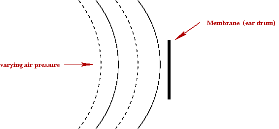
A basic desciption of how sound works:

In brief: air moves your eardrum, which in turns causes a chain of events inside the ear that results in neural signals and perception of sound.
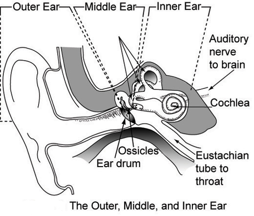
We can abstract this as a membrane that is made to move by changing patterns in air pressure.
How do we make sense of "sound" beyond this high-level description?
- Eventually, we want "sound" as input to algorithms that "process" sound.
- We need a model of "sound" that results in numbers that can be processed.
- One idea: what about volume?
  In-Class Exercise 2: Suppose we somehow record "volume" levels of sound. Is that enough to characterize sound? Why or why not?
To better understand quantitative models of sound, it's easier to work in reverse: see what causes sound.
- A speaker is the opposite of the eardrum (or microphone): electric current is used to move a stiff membrane that then moves air:
- We can quantify the movement (displacement) of the membrane:
  
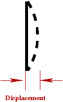
  Let $f(t)$ = the displacement at time $t$
- Values of $f(t)$ could serve as our model for sound.

In-Class Exercise 3: Let's see what we get if we set $f(t)=100$ for various values of $t$:

What does the function look like when plotted?

Add code to MakeSound.java to set $f(t)=100$ and play the sound. What do you hear? Explain.

In-Class Exercise 4: Next, examine MakeSound2.java:

Add code to print the byte values to screen. Compile and execute. What do you notice about the output ($f(t)$) values?

Compile and execute MakeSound3.java to view the function $f(t)$. Does it look familiar?

In-Class Exercise 5: Now let's make some music. Modify the code in MakeMusic.java to create some music.

At this point, several questions arise:

We know that we can make music (a kind of sound) out of sinusoids. Is all music like that?
Are other functions possible? What kinds of $f(t)$ correspond to sounds.
We were thinking of $f(t)$ as a continuous function (one value for each possible $t$. But the samples were discrete (in an array). How to make sense of this?

In-Class Exercise 6: Find a picture of digitized sound on the internet. See if you can make sense of it.

In-Class Exercise 7: Study the code in MakeSound4.java. Then compile and execute. What do you notice about the first two curves? How does the third relate to the first two?

13.2 Sines and cosines

Let's review the sin and cosine functions:

What are $\sin$ and $\cos$?
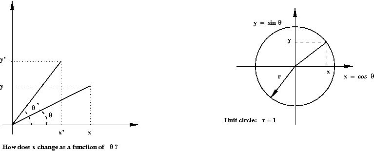
- Note that they are functions.
  → For a variable $t$, the function $\sin(t)$ is well-defined.
Convention: measure angle in radians where a radian is defined such that $2\pi$ radians = $360^\circ$.
Important: $\sin(t)$ is defined for all $t$.

In-Class Exercise 8: Let's explore the last point.

Note: $2\pi$ is approximately $6.29$. Why is it OK to define a value for $\sin(17.5)$ or $\sin(-156.32)$? How are these values defined?

Compile and execute PlotSin.java to plot the function $\sin$ and $\cos$ in the range $[0,20]$. How many times does the function "repeat" in this range.

Next, let's understand the concept of frequency:

In English: it refers to "how often"
→ There is an implied notion of time.
For a sinusoid like $\sin(t)$, it means "how often the function repeats itself per unit time".
To understand this better, let's see what a cycle means:
- Since $\sin(t + 2\pi) = \sin(t)$, the crest-and-trough shape repeats.
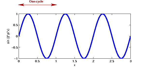
- A single crest-and-trough is called a cycle.
The frequency is the number of cycles per unit time.
→ The unit of measurement is called a Hz (Hertz), the number of cycles per unit time.
Let's examine the function $\sin(2\pi\omega t)$.
In-Class Exercise 9: Compile and execute PlotSin2.java to plot $\sin(2\pi\omega t)$ in the range $[0,1]$ with $\omega = 1, 2, 3$. What is the relationship between the three curves?
Thus, $\omega$ is the frequency: the number of cycles per second.
Note: $\omega$ can be a real number.
→ You can have a frequency of 3.356 cycles per second.
The function $\sin(2\pi k \omega t)$, for integer $k$, is called a harmonic of $\sin(2\pi \omega t)$
→ $k$ cycles of $\sin(2\pi k \omega t)$ fit into one single cycle of $\sin(2\pi \omega t)$
The inverse of frequency is called the period, the length of time for one complete cycle.

We'll next look at phase:

You can shift a sin wave by adding a fixed constant to the argument: $\sin(2\pi \omega t + \phi )$.

In-Class Exercise 10: Modify PlotSin3.java to plot $\sin(2\pi t + \phi )$ in the range $[0,1]$. Plot four separate curves with $\phi =0, \pi /4, \pi /2, \pi $. What can you say about $\sin(2\pi t + \pi /2)$? Similarly, plot $\cos(2\pi t + \pi /2)$ and comment on the function.

Finally, the third parameter to a sinusoid is its amplitude:

First, note that multiplying a sinusoid by a constant, e.g., $\alpha \sin(t)$ does not change the period.
In-Class Exercise 11: Why?
The amplitude is the peak height of a sinusoid.
→ Since the maximum value of $\sin(t)$ is 1.0, the amplitude of $\alpha \sin(t)$ is $\alpha $.
Thus, a complete sin function is written as $\alpha \sin(2\pi \omega t + \phi )$
→ with amplitude $\alpha $, frequency $\omega $ and phase $\phi $.

We will now see what happens when we add sinusoids.

First, let's plot the sum of two simple sine's:
In-Class Exercise 12: Consider the two functions $sin(2\pi t)$ and $\sin(4\pi t)$. Draw these by hand on paper (roughly) for $t$ in the range $[0,1]$ and try to draw the shape of their sum $\sin(2\pi t) + \sin(4\pi t)$. Compile and execute SinSum.java, and compare with your drawing.
In the above example, we added two harmonics. What is the resulting sound when we add two harmonics?
In-Class Exercise 13: Compile and execute MakeSound5.java. Then, hear the two frequencies one by one. Are you able to tell the difference?
Beyond frequency (roughly, pitch) and amplitude (roughly, loudness), sound also has texture:
- Texture is harder to characterize.
  → A "C" note on a piano sounds different than the same note on a violin. Why?
- One way to create texture is to add harmonics.
- Another way: vary the amplitude of the harmonics during a short interval
  → called wave shaping
- In practice, a single note (instrument or voice) is a complex sound.
Let's return to elementary sinusoids and observe what happens when we add a number of harmonics.
In-Class Exercise 14: Consider the sum $$ \sum_k \frac{1}{k} \sin(2\pi kt) $$ where $k=1, 3, 5, ...$ etc. This is a sum of odd harmonics. Compile and execute SinSum2.java, which shows the sum of the first two odd harmonics. Change the code to compute the sum of the first six old harmonics (where $k=11$ is the last term).
It can be shown that the (weighted) sum of odd harmonics approximates a square wave as closely as desired.

13.3 Fourier's question (and answer)

The above approximation of a square wave with sums-of-sines raises an intriguing question: can any function be approximated by a sum of sinusoids?

This was the question raised by Joseph Fourier in the 18th century (when working on problems related to modeling heat transfer).

In-Class Exercise 15: Unfortunately, $\sin$ functions alone aren't enough. Can you think of a function that no weighted sum of $\sin$ functions could possibly approximate?

It would be many years before it could be rigorously shown that any continuous function $f(t)$ with period $T$ can be expressed as $$ f(t) \eql a_0 \plss \sum_{k} a_k \sin(\frac{2\pi kt}{T}) \plss \sum_{k} b_k \cos(\frac{2\pi kt}{T}) $$ where $a_k$ and $b_k$ are real numbers.

This is one form of the celebrated Fourier Series theorem. Note:
- Fourier himself was ignored when he presented this idea in 1807 (without a rigorous proof).
- Various mathematicians proved versions of this over the next 100+ years, with fewer assumptions.
- What's remarkable: the same basic frequency ($\omega =1$) and harmonics are the only frequencies, and they are all in phase.
  → The only parameters are the amplitude constants $a_k$.
- The sum is a linear combination of sinusoids
  → This will turn out to have great significance, not just practically, but also theoretically.
- Fourier analysis is now a large topic by itself, with both theory and applications that go well beyond understanding sound.
How does one calculate the constants $a_k$? More about that later.
Although the above result is remarkable, is it really useful for our purposes (analyzing sound)?
- The weighted sum is a continuous function.
  → Digitized sound is a collection of discrete values.
- Even if we could approximate digitized sound with a continuous function we don't know "the function" ahead of time
  → e.g., we don't have a function that describes the Star-Spangled Banner.

13.4 Digitized sound

Consider a digitized sinusoid:

When analog sound is recorded digitally, the analog sound is sampled at equally-spaced times.
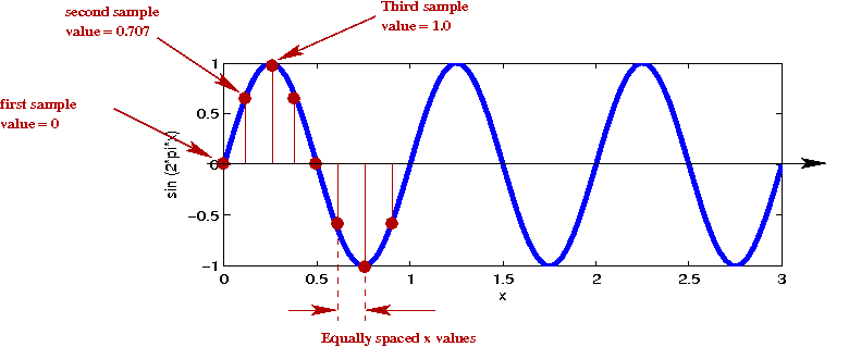
Example: standard digital audio (on a CD) is sampled approximately 44,100 times in a second (44.1 kHz).
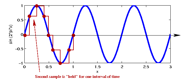
During playback, the analog output is constructed from digital samples, and is approximated by a step function - the value of the sinusoid at $N$ equally-spaced discrete points.
→ $N$ samples.

In-Class Exercise 16: Compile and execute Sampling.java, which shows 10 samples taken from $\sin(2\pi kx)$. Try $k=1, 2, ..., 5$ and $k=8$. At what values of $k$ do 10 samples become insufficient?
The Nyquist sampling theorem: the sampling rate needs to be at least twice the frequency of the highest-frequency present in the signal.
- 20,000 Hz is considered the highest audible frequency
  → About 40 kHz should be sufficient.
- What is interesting: you don't need much more than twice-the-highest frequency.
Note: the sampling rate (the number of samples/second) discretizes the time axis.
The signal axis is also discretized
→ A fixed number of bits are used to represent each signal value.
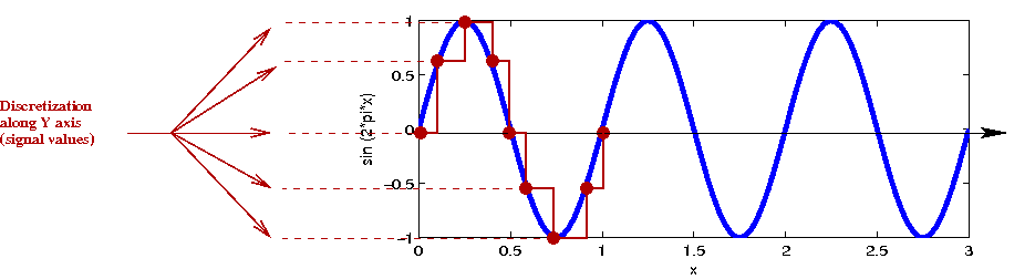
Example: 16-bit audio uses 16 bits to represent $2^{16}$ possible values.

To summarize:

In digitized sound, the signal consists of samples taken at equally spaced intervals.
Each sample is a number
→ The strength of the signal at that time.
This "signal strength" can itself take on a finite number of values (e.g., $2^{16}$).
For theory purposes, we can treat the signal value as continuous because, in practice, 16 or 24 bits is plenty for the signal values.
Our real goal: given an audio file (a collection of digital audio samples), identify the frequencies present and possibly manipulate the content (filtering).
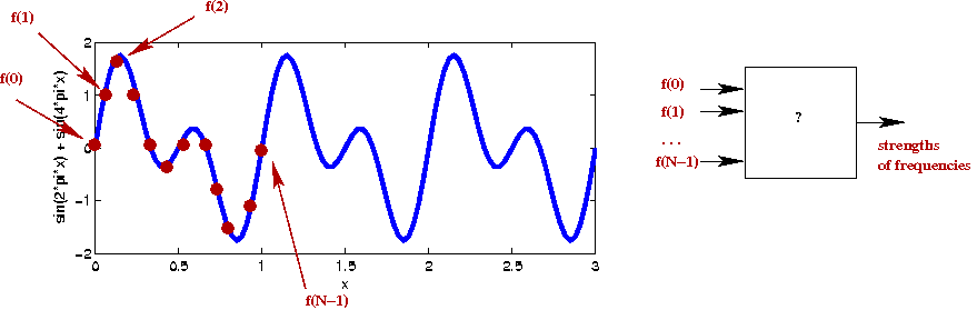
Think of the signal as $m$ numbers $f(0), f(1), ..., f(m-1)$.
→ we want an algorithm to take these $m$ numbers and tell us something about the frequency content.
One approach: use Fourier series
- Approximate signal using a piecewise-linear function on samples.
- Then, compute coefficients in Fourier series.
- This tells you the "strength" of each frequency.
- Next: adjust the strength of some frequencies and convert back to sound
  → e.g., bass/treble control (equalizer).
Unfortunately, computing the coefficients is extremely complicated and time consuming.
- For $N$ samples and $M$ sinusoids, this requires $O(MN)$ integrations.
- Each integration itself is an iteration.
  → $O(N^2)$ integrations (if $M$ is as large as $N/2$).
Solution: a direct approach
→ The Discrete Fourier Transform (DFT)
To understand the DFT, we need a little background in complex numbers.

13.5 Complex numbers

What are they and where did they come from?

Consider an equation like $x^2 = 4$.
→ We know that $x = \pm 2$.
What about $x^2 = 2$?
→ Doesn't change the concept: $x = \pm \sqrt{2}$.
However, $x^2 = -2$ poses a problem.
Suppose we define the "number" $\sqrt{-1}$ and give it a symbol: $$ i \eql \sqrt{-1} $$
Then $$ (i \sqrt{2})^2 \eql i^2 (\sqrt{2})^2 \eql (\sqrt{-1})^2 (\sqrt{2})^2 \eql -2 $$ gives a solution to the previous equation.
In general, a complex number is written as $a + ib$ where $a$ and $b$ are real numbers.
- The $a$ in $a+ib$ is called the real part.
- $b$ is called the imaginary part.
Once we define complex numbers, there are many ways in which we could define the basic operations of addition, multiplication etc.
- Obviously, one would like complex numbers to be more general than real numbers
  → Operations defined on complex numbers should give the expected results when applied to complex numbers with only real parts.
- It turns out, to make things consistent, we need to define addition and multiplication (subtraction and division follow from these) as follows:
  - $ (a+ib) + (c+id) \defn (a+c) + i(b+d)$
  - $ (a+ib)(c+id) \defn (ac-bd) + i(ad+bc) $
Once arithmetic has been defined, we can define functions on complex numbers
→ e.g., for a complex number $z$, define $f(z) = z^2$
What about $\sin(z)$? Does it make sense?
In-Class Exercise 17: What do you think?

Polar representation of complex numbers:

One useful graphical representation is obvious when we write complex number $z$ as $z = x + iy$.
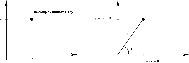
Given this, one can easily write $$ \eqb{ z & \eql & x + iy \\ & \eql & r \cos(\theta) + i r\sin(\theta)\\ & \eql & r (\cos(\theta) + i \sin(\theta)) } $$
An important observation made by Euler:
Suppose you define $$ e^z \eql 1 + z + \frac{z^2}{2!} + \frac{z^3}{3!} + \ldots $$ analogous to the real function $e^x$: $$ e^x \eql 1 + x + \frac{x^2}{2!} + \frac{x^3}{3!} + \ldots $$
Then $$ \eqb{ e^{i\theta} & \eql & 1 + (i\theta) + \frac{(i\theta)^2}{2!} + \frac{(i\theta)^3}{3!} + \ldots \\ & & \mbox{... some algebra ...} \\ & \eql & \mbox{series for $\cos(\theta)$} \plss i (\mbox{series for $\sin(\theta)$}) \\ & \eql & \cos(\theta) + i\sin(\theta) } $$ → called Euler's relation.
Thus, $$ z \eql r e^{i \theta} $$ is the polar representation of the complex number $$ z \eql x + iy \eql r (\cos(\theta) + i\sin(\theta)) $$
Observe: when $r=1$, and $\theta=2\pi$ or $\theta=-2\pi$ $$ e^{2\pi i} \eql 1 \eql e^{-2\pi i} $$
Next, $$ (e^{\frac{2\pi i}{N}})^N \eql 1 $$ Similarly, $$ (e^{-\frac{2\pi i}{N}})^N \eql 1 $$
In particular, this means that $e^{\frac{2\pi i}{N}}$ and $e^{-\frac{2\pi i}{N}}$ are $N$-th roots of unity.
We will use the notation $$ \eqb{ W_N & \eql & e^{\frac{2\pi i}{N}} \\ W_N^* & \eql & e^{-\frac{2\pi i}{N}} } $$
Lastly, because $\cos(-x)=\cos(x)$ and $\sin(-x)=-\sin(x)$ $$ e^{-\frac{2\pi i}{N}} \eql \cos(\frac{2\pi}{N}) - i \sin(\frac{2\pi}{N}) $$

To summarize: $$ \eqb{ W_N & \eql & e^{\frac{2\pi i}{N}} \eql \cos(\frac{2\pi}{N}) + i \sin(\frac{2\pi}{N}) \\ W_N^* & \eql & e^{-\frac{2\pi i}{N}} \eql \cos(\frac{2\pi}{N}) - i \sin(\frac{2\pi}{N}) } $$

An even shorter take-away:

There are two special complex numbers called $W_N$ and $W_N^*$.
Both will play an important role in defining the Fourier transform.

Note: we will sometimes write $W_N^*$ as $W_{*N}$ when we need more space for superscripts.

Implementing complex numbers:

We will use a simple object to represent a complex number, for example:

public class Complex {

    // Real and imaginary parts
    double re, im;

    public Complex (double re, double im)
    {
        this.re = re;
        this.im = im;
    }

    public Complex add (Complex c)
    {
        return new Complex (re + c.re, im + c.im);
    }

    public Complex mult (Complex c)
    {
        return new Complex (re*c.re - im*c.im, re*c.im + im*c.re);
    }

}

With this, we can write code like:

        // Make one complex number (recognize this one?):
        Complex c1 = new Complex (Math.cos(2*Math.PI/N), -Math.sin(2*Math.PI/N));

        // Make another:
        Complex c2 = new Complex (1, 0);

        // Multiply:
        Complex result = c1.mult (c2);

13.6 The Discrete Fourier Transform

Let's start with the input to the algorithm:

From an engineering viewpoint, this is easy: the input consists of $N$ real numbers $f(0), f(1), ..., f(N-1)$.
→ These are $N$ digitized samples of the sound signal.
But there are two questions we need to address:
1. What is $N$?
2. We sense that we are going to compute with complex numbers
  → How do we convert to complex?
First, the value of $N$:
- At 44,100 samples/second, we need $N = 44100 * 60 * 3 = 7,938,000$ for a 3-minute song (assuming one channel).
- Even for an efficient algorithm, this is too large a value of $N$ in practice.
- Solution: segment the samples into a number of "windows" with a small $N$.
- Example, with $N=1024$, we'd need $7,938,000 / 1024 = 7752$ windows.
  → This raises another problem: correlating our analysis across the different windows.
- Generally, small windows are desirable because the sound (music) is often changing.
Next, the $N$ samples $f(0), f(1), ..., f(N-1)$ are real numbers. How do we make them complex?
→ Easy: treat these as complex numbers with $0$ as the imaginary part.
- Example: the real number $3.64$ is the complex number $(3.64, 0)$.
Henceforth, we'll assume the samples $f(0), f(1), ..., f(N-1)$ are complex.

Now, the output:

The output is going to be $N$ complex numbers $F(0), F(1), ..., F(N-1)$.
To summarize:

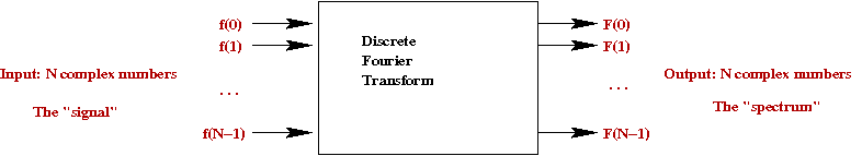
The Discrete Fourier Transform (DFT):

The complex numbers $F(0), F(1), ..., F(N-1)$ are computed as follows: $$ \eqb{ F(k) & \eql & \frac{1}{N} \sum_j f(j) (e^{-2\pi i/N})^{kj} \\ & \eql & \frac{1}{N} \sum_j f(j) ({W_N^*}^{k})^j \\ & \eql & \frac{1}{N} \left( f(0) ({W_N^*}^{k})^0 + f(1) ({W_N^*}^{k})^1 + f(2) ({W_N^*}^{k})^2 + \ldots + f(N-1) ({W_N^*}^{k})^{N-1} \right) \\ } $$
Think of this as: a particular $F(k)$ value is a weighted sum of all $N$ samples
→ Here, the weights are different powers of ${W_N^*}^{k}$.
It turns out that one can recover the original samples from the DFT values: $$\eqb{ f(j) & \eql & \sum_k F(k) (e^{2\pi i/N})^{jk} \\ & \eql & \sum_k F(k) (W_N^{j})^k \\ & \eql & F(0) W_N^0 + F(1) W_N^j + F(2) W_N^{2j} + \ldots + F(N-1) W_N^{(N-1)j} }$$
This is called the inverse DFT.
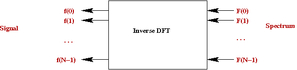
The transform and inverse transforms are very alike, except for:
- One uses $W_N^*$ and the other uses $W_N$.
- There's no $\frac{1}{N}$ scaling term in the inverse.
The two $N$-th roots can be swapped (you get a slightly different transform, but it still works, and some books use this definition).
About the scaling term:
- The scaling term comes out of the math (see later).
- As an alternative, one can define use the $\frac{1}{N}$ term in the inverse-DFT, but not in the DFT.
  → Some books define it this way.
- One can also "split the difference" and use a $\frac{1}{\sqrt{N}}$ term in both.
Note: all arithmetic operations above are complex arithmetic operations.
Some terminology:
- signal: the $N$ (input) numbers $f(0), f(1), ..., f(N-1)$.
- spectrum: the $N$ (output) numbers $F(0), F(1), ..., F(N-1)$.

Next, let's write code to implement the DFT:

High-level pseudocode (with complex-number arithmetic):

Algorithm: DFT (f, N)
Input: the signal f[0],..,f[N-1] and size N
1.    W*_N = cos(2π/N) - i sin(2π/N)
2.    for k=0 to N-1
3.        sum = 0
4.        for j=0 to N-1
5.            sum = sum + f[j] W*_N^kj  // Note: we are raising W*_N to the kj-th power.
6.        endfor
7.        F[k] = 1/N * sum
8.    endfor
9.    return F

In-Class Exercise 18: Before proceeding, can you identify the complex arithmetic operations above? How many are there?

The above algorithm is slightly inefficient if we compute ${W_N^*}^{kj}$ directly using complex arithmetic.
Instead, we will compute $$ \eqb{ {W_N^*}^{kj} & \eql & e^{-2\pi ikj/N} \\ & \eql & \cos(2\pi kj/N) + i \sin (2\pi kj/N) } $$

Next, let's see what this looks like in Java:

    public static Complex[] DFT (Complex[] signal, int N) 
    {
	// Make the space for the resulting DFT (the spectrum).
	Complex[] spectrum = new Complex [N];

	// Compute the DFT
	for (int k=0; k<N; k++) {
	    Complex sum = new Complex (0,0);
	    for (int j=0; j<N; j++) {
		// Compute W*_N^kj:
		double cosTerm = Math.cos (2*Math.PI*k*j / (double)N);
		double sinTerm = -Math.sin (2*Math.PI*k*j / (double)N);
		Complex WN_star_pow_kj = new Complex (cosTerm, sinTerm);
		// Multiply by f(j):
		Complex product = signal[j].mult (WN_star_pow_kj);
		// Accumulate:
		sum = sum.add (product);
	    }
	    // Scale by N:
	    spectrum[k] = sum.mult (1.0/N);
	}

	return spectrum;
    }

Note: we need to convert a real signal into complex form (with $0$ as the imaginary part).

The inverse DFT is very similar. Here's pseudocode, written in the more efficient way:

Algorithm: inverse-DFT (F, N)
Input: the spectrum F[0],..,F[N-1] and size N
1.    for j=0 to N-1
2.        sum = 0
3.        for k=0 to N-1
4.            w = cos (2πjk/N) + i sin (2πjk/N)
5.            sum = sum + F[n] w                   // w = W_N^jk
6.        endfor
7.        f[j] = sum
8.    endfor
9.    return f     // The signal

Note: the signal is in complex form.
→ The usable part is the real part of this complex array.
Both the DFT and inverse-DFT take time $O(N^2)$.

13.7 Using the Discrete Fourier Transform

Recall our overall goal: to extract the "frequency content" of digitized audio and possibly manipulate that content.

Unfortunately, it's not as straightforward as applying the DFT to digitized audio.
We first need to understand how to "read" frequency content in a DFT spectrum.
First, at a basic level, let's recall what the DFT does: it takes $N$ input numbers (the signal)
$f(0), f(1), ..., f(N-1)$
and computes $N$ output numbers (the spectrum)
$F(0), F(1), ..., F(N-1)$
In an audio application, the $N$ input numbers are real values (amplitudes) of the audio signal taken at $N$ equally spaced times.
We don't yet know how to interpret the output (complex) numbers.
The first thing to realize is that: you can compute the DFT of any bunch of numbers
→ any $N$ numbers will result in a DFT spectrum, whatever the origin of those numbers.
Even if the source is digitized audio, the "frequency" content of the DFT spectrum may or may not correspond to the "frequency" content of the original audio
→ It's up to us to make the correspondence work.
This is not always straightforward
→ For example, if the sampling was not performed at a high enough frequency, it will fail (The DFT output won't make sense).

Let's start with a little exploration:

One of the best ways of understanding the DFT output is to start with some DFT output and apply the inverse-DFT to see what "signal produces this output".
Perhaps the simplest such exercise is to set $F(k) = C$ for some $k$ and the rest $F(i) = 0$.
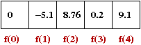
In-Class Exercise 19: The code in TestDFT.java sets $F(k)=C$ and displays both spectrum and reverse-engineered signal. Try $k=0,1,2$ and then $k=7,6$. What do you notice?
What did we learn?
- $F(0)=C$ arises from a constant (unvarying, or zero-frequency) signal
  → Sometimes this is called the "DC" content of the signal.
- The inverse-DFT results in non-zero imaginary signal numbers
  → We only examine the real part of the signal.
- Although the signals above varied (had frequency content), the resulting signals did not resemble the sine's and cosine's we'd seen earlier.
It will help to use a larger value of $N$.
In-Class Exercise 20: Use TestDFT2.java to $F(k)=C$. Try $k=0,1,2$ and then $k=63,32$. At what value of $k$ do you see the highest frequency?
At last we see a real sine wave.
The following summarizes a few points we learned above:
- Once again, $F(0)=C$ results from a "pure DC" (all constant) signal.
- The lowest frequencies occur at the ends of the spectrum: $F(1), F(N-1)$.
- The highest frequencies occur towards the middle.
- So far, we've only seen cosine's in the real part of the signal
- If the input signal is a digitized sinusoid, one is led to believe that the spectrum will have a singularity.
Our spectrum did not have any imaginary content.
→ This raises the question: do real signals produce imaginary numbers in the spectrum?

Next, let's start with a known sinusoid and examine the resulting spectrum.

In-Class Exercise 21: Use TestDFT3.java to explore the spectrum of different sinusoids:

For sine's, try freq = 1, 2, ..., N/2.

For cosine's try freq = 1,2, ..., N/2.

What did we learn?

The sine's result in a split imaginary spectrum of different signs:
→ For example: when the frequency is 1, we get $F(1)=(0,-C/2)$ and $F(N-1)=(0,C/2)$.
The pure cosine's result in a split real spectrum of the same sign:
→ For example: when the frequency is 1, we get $F(1)=(C/2,0)$ and $F(N-1)=(C/2,0)$.
The DFT captures frequency content in the input numbers
→ The lowest frequency is when all $N$ numbers represent a single cycle of the sinusoid.
The highest possible frequency is $N/2$, but only for a cosine.

We can summarize the results for sine's in the following table:

frequency	Spectrum
1	F(1)=(0,-C/2), F(N-1)=(0,C/2)
2	F(2)=(0,-C/2), F(N-2)=(0,C/2)
3	F(3)=(0,-C/2), F(N-3)=(0,C/2)
. . .
N/4	F(N/4)=(0,-C/2), F(N-N/4)=(0,C/2)
. . .
N/2+1	F(N/2+1)=(0,-C/2), F(N-N/2-1)=(0,C/2)

Similarly, for cosine's:

frequency	Spectrum
1	F(1)=(C/2,0), F(N-1)=(C/2,0)
2	F(2)=(C/2,0), F(N-2)=(C/2,0)
3	F(3)=(C/2,0), F(N-3)=(C/2,0)
. . .
N/4	F(N/4)=(C/2,0), F(N-N/4)=(C/2,0)
. . .
N/2	F(N/2)=(C,0)

What about combining sinusoids?

Let us combine two sinusoids and examine the resulting spectrum:
In-Class Exercise 22: Use TestDFT4.java to explore the spectrum of combined sinusoids.
Thus, we see that the DFT very nicely teases out the different frequencies.

Finally, let's use what we've learned in an audio application:

We will write code to filter out high frequencies.
Let's do this in two stages: (1) first with sine's; (2) then with real audio.
Recall that the high frequenies were near the center
→ Accordingly, as an approximation we will simply zero-out the frequency content in the "center" of the spectrum.
In-Class Exercise 23: Compile and execute TestDFT5.java. Examine the code to see how filtering was achieved by manipulating the spectrum.
Next, we want to apply this to audio.
Recall that the number of samples is more than 120,000 for 3 seconds of audio (at 44,100 samples per second).
→ Should we use $N$ = total number audio samples?
There are at least two reasons we should not:
- First, the computation time (recall: the DFT takes $O(N^2)$ time).
- More importantly, audio is often changing in time
  → It's better to apply the DFT to short intervals.
Let us use $N=1024$ and apply this repeatedly.
- That is, apply the filter to the first $N$ samples $f(0), ..., f(N-1)$
  → the first window.
- Then, apply the filter to the next $N$ samples $f(N), ..., f(2N-1)$.
  → the second window.
- ... and so on. Then, construct the final filtered signal by stitching together the different signal windows.
In-Class Exercise 24: Compile and execute TestDFT6.java.
We will next study the faster FFT algorithm.

13.8 The Fast Fourier Transform

Key ideas:

Like other $O(N^2)$ algorithms we've encountered, we need to ask: is there a divide-and-conquer strategy that will give us an $O(N \log N)$ algorithm?
The answer is yes, but we're going to have to "unfurl" the sum to understand how this can be done. And there are some complications to deal with.
We will use $N=8$ in a running example.
Let's start, for example, by looking at how $F(3)$ (one of the spectral terms) is computed with the DFT: $$\eqb{ F(3) & \eql & f(0) W_{*N}^{3\times 0} + f(1) W_{*N}^{3\times 1} + f(2) W_{*N}^{3\times 2} + \ldots + f(N-1) W_{*N}^{3(N-1)} \\ & \eql & f(0) (W_{*N}^3)^0 + f(1) (W_{*N}^3)^1 + f(2) (W_{*N}^3)^2 + \ldots + f(N-1) (W_{*N}^3)^{(N-1)} \\ }$$
Here, we've emphasized the fact that, for the $F(k)$ term, we get a weighted sum of powers of $W_{*N}^3$.
Next, we are going to re-order the terms (for our $N=8$ example) to separate out even and odd powers: $$\eqb{ F(3) & \eql & f(0) (W_{*N}^3)^0 + f(2) (W_{*N}^3)^2 + f(4) (W_{*N}^3)^4 + f(6) (W_{*N}^3)^6 + \\ & & f(1) (W_{*N}^3)^1 + f(3) (W_{*N}^3)^3 + f(5) (W_{*N}^3)^5 + f(7) (W_{*N}^3)^7 \\ }$$
Now, it would be nice if the even terms reduced to a DFT of size N/2, and likewise for the odd terms.
→ But this is not (yet) the case.
Observation 1: $ (W_{*N}^k)^{2n} \eql (W_{*N/2}^k)^{n} $
In-Class Exercise 25: Why?
With this key observation, $$\eqb{ F(3) & \eql & f(0) (W_{*N/2}^3)^0 + f(2) (W_{*N/2}^3)^1 + f(4) (W_{*N/2}^3)^2 + f(6) (W_{*N/2}^3)^3 + \\ & & W_{*N}^3 \left( f(1) (W_{*N/2}^3)^0 + f(3) (W_{*N/2}^3)^1 + f(5) (W_{*N/2}^3)^2 + f(7) (W_{*N/2}^3)^3 \right)\\ }$$

The powers used are exactly what are used in the size-$N/2$ problem!
→ It now looks like we have a candidate for recursion.
However, it's not so simple, as we'll see.
First, let's recap what we have: $$\eqb{ F(3) & \eql & \mbox{ size N/2 DFT computed with } f(0),f(1),f(2),f(3) \;\;+\;\; \\ & & W_{*N}^3 \left( \mbox{ size N/2 DFT computed with } f(0),f(1),f(2),f(3) \right)\\ }$$

Thus, the following recursion works:

Algorithm: DFT2 (f, N)
Input: the signal f[0],..,f[N-1] and size N
1.    for k=0 to N-1
2.        F[k] = 1/N * recursiveDFT (f, N, k)
3.    endfor
4.    return F

Algorithm: recursiveDFT (f, N, k)
Input: the signal f[0],..,f[N-1], size N, and a subscript k
      // Compute  \(W*_N^k\)
1.    w = cos(2πk/N) - i sin cos(2πk/N)
      // Bottom-out case:
2.    if N = 2
3.        return f[0] + w f[1]
4.    endif
      // Divide and conquer.
5.    even_f = f[0], f[2], ..., f[N-2]
6.    odd_f = f[1], f[3], ..., f[N-1]
7.    return recursiveDFT(even_f, N/2, k)  +  w * recursiveDFT(odd_f, N/2, k)

Unfortunately, this still takes $O(N^2)$ time.
In-Class Exercise 26: Why?
What we need: once a smaller-size DFT is computed, we should never come back to that size.

We're going to need more insight and use one more property of $W_{*N}$ to make this work:

First, let's return to our size-$N$ for $N=8$:
- What is the full DFT for this?
- It's a list of $N=8$ complex numbers: $F(0), F(1), ..., F(7)$.
- Here, the $k$-th term can be written as: $$\eqb{ F(k) & \eql & f(0) (W_{*N/2}^k)^0 + f(2) (W_{*N/2}^k)^1 + f(4) (W_{*N/2}^k)^2 + f(6) (W_{*N/2}^k)^3 + \\ & & W_{*N}^k \left( f(1) (W_{*N/2}^k)^0 + f(3) (W_{*N/2}^k)^1 + f(5) (W_{*N/2}^k)^2 + f(7) (W_{*N/2}^k)^3 \right)\\ }$$
Next, suppose we have already (somehow) computed the size-$N/2$ DFT's for the even and odd signal values.
- What do these look like?
- The size-$N/2$ DFT for $f(0), f(2), f(4), f(6)$ will be four numbers, let's call them $G(0), G(1), G(2), G(3)$: $$\eqb{ G(0) & \eql & f(0) (W_{*N/2}^0)^0 + f(2) (W_{*N/2}^0)^1 + f(4) (W_{*N/2}^0)^2 + f(6) (W_{*N/2}^0)^3 + \\ G(1) & \eql & f(0) (W_{*N/2}^1)^0 + f(2) (W_{*N/2}^1)^1 + f(4) (W_{*N/2}^1)^2 + f(6) (W_{*N/2}^1)^3 + \\ G(2) & \eql & f(0) (W_{*N/2}^2)^0 + f(2) (W_{*N/2}^2)^1 + f(4) (W_{*N/2}^2)^2 + f(6) (W_{*N/2}^2)^3 + \\ G(3) & \eql & f(0) (W_{*N/2}^3)^0 + f(2) (W_{*N/2}^3)^1 + f(4) (W_{*N/2}^3)^2 + f(6) (W_{*N/2}^3)^3 + \\ }$$
  In-Class Exercise 27: It's worth spending a few minutes verifying this; there are a lot of sub- and superscripts to keep track of.
- Similarly, the size-$N/2$ DFT for $f(1), f(3), f(5), f(7)$ will be four numbers: $H(0), H(1), H(2), H(3)$. $$\eqb{ H(0) & \eql & f(1) (W_{*N/2}^0)^0 + f(3) (W_{*N/2}^0)^1 + f(5) (W_{*N/2}^0)^2 + f(7) (W_{*N/2}^0)^3\\ H(1) & \eql & f(1) (W_{*N/2}^1)^0 + f(3) (W_{*N/2}^1)^1 + f(5) (W_{*N/2}^1)^2 + f(7) (W_{*N/2}^1)^3\\ H(2) & \eql & f(1) (W_{*N/2}^2)^0 + f(3) (W_{*N/2}^2)^1 + f(5) (W_{*N/2}^2)^2 + f(7) (W_{*N/2}^2)^3\\ H(3) & \eql & f(1) (W_{*N/2}^3)^0 + f(3) (W_{*N/2}^3)^1 + f(5) (W_{*N/2}^3)^2 + f(7) (W_{*N/2}^3)^3\\ }$$
To summarize: from these 8 numbers
$G(0), G(1), G(2), G(3), H(0), H(1), H(2), H(3)$
we'd like to compute the 8 size-$N$ DFT numbers:
$F(0), F(1), F(2), F(3), F(4), F(5), F(6), F(7)$.
Consider $F(3)$, for example:
- Is it true that we can compute $F(3)$ from $G(3)$ and $H(3)$?
- Let's see ... $$\eqb{ G(3) + W_{*N}^3 H(3) & \eql & f(0) (W_{*N/2}^3)^0 + f(2) (W_{*N/2}^3)^1 + f(4) (W_{*N/2}^3)^2 + f(6) (W_{*N/2}^3)^3 \;\; + \\ & & W_{*N}^3 \left( f(1) (W_{*N/2}^3)^0 + f(3) (W_{*N/2}^3)^1 + f(5) (W_{*N/2}^3)^2 + f(7) (W_{*N/2}^3)^3 \right)\\ & \eql & f(0) (W_{*N/2}^3)^0 + f(1) (W_{*N}^3)^1 + f(2) (W_{*N}^3)^2 + \ldots + f(7) (W_{*N}^3)^7 }$$
So, it appears the answer is yes.
However, consider $F(5)$:
- First, we can't do
  $F(5) = G(5) + W_{*N}^5 H(5)$
  because there's no such thing as $G(5)$ or $H(5)$.
- Instead, consider
  $G(1) + W_{*N}^5 H(1)$
- Why $G(1)$ and $H(1)$?
         → The hope is that
               $G(0),H(0)$ can be used for $F(4)$
               $G(1),H(1)$ can be used for $F(5)$
               $G(2),H(2)$ can be used for $F(6)$
               $G(3),H(3)$ can be used for $F(7)$
OK, back to $F(5)$. Let's see what $G(1)$ and $H(1)$ produce: $$\eqb{ F(1) + W_{*N}^5 H(1) & \eql & f(0) (W_{*N/2}^1)^0 + f(2) (W_{*N/2}^1)^1 + f(4) (W_{*N/2}^1)^2 + f(6) (W_{*N/2}^1)^3 \;\; + \\ & & W_{*N}^5 \left( f(1) (W_{*N/2}^1)^0 + f(3) (W_{*N/2}^1)^1 + f(5) (W_{*N/2}^1)^2 + f(7) (W_{*N/2}^1)^3 \right)\\ & \eql & f(0) + f(1) W_{*N}^5 + f(2) W_{*N}^2 + f(3) W_{*N}^2 W_{*N}^5 + \\ & & f(4) W_{*N}^4 + f(5) W_{*N}^5 W_{*N}^4 + f(6) W_{*N}^6 + f(7) W_{*N}^5 W_{*N}^6 }$$
Now compare this with what is desired: $$\eqb{ F(5) & \eql & f(0) + f(1) (W_{*N}^5) + f(2) (W_{*N}^5)^2 + f(3) (W_{*N}^5)^3 + f(4) (W_{*N}^5)^4 + f(5) (W_{*N}^5)^5 + f(6) (W_{*N}^5)^6 + f(7) (W_{*N}^5)^7 }$$
- This works out fine for the even terms.
- But the odd terms don't look right.
- For example, comparing the coefficients of $f(3)$ in each, one wonder if $$ W_{*N}^2 W_{*N}^5 \eql (W_{*N}^5)^3? $$
- Luckily, the answer is yes.
Observation 2: $$ W_{*N}^k \eql W_{*N}^{k \mod N} $$
In-Class Exercise 28: This is easy to prove - try it.
To summarize (for $N=8$):
- For $F(0), F(1), F(2), F(3)$:
         $F(0) = G(0) + W_{*N}^5 H(0)$
         $F(1) = G(1) + W_{*N}^5 H(1)$
         $F(2) = G(2) + W_{*N}^5 H(2)$
         $F(3) = G(3) + W_{*N}^5 H(3)$
- Or, more succinctly, for $k=0,..,3$:
  $F(k) = G(k) + W_{*N}^5 H(k)$
- While, for $F(4), F(5), F(6), F(7)$:
         $F(4) = G(0) + W_{*N}^5 H(0)$
         $F(5) = G(1) + W_{*N}^5 H(1)$
         $F(6) = G(2) + W_{*N}^5 H(2)$
         $F(7) = G(3) + W_{*N}^5 H(3)$
- Or, more succinctly, for $k=4,..,7$:
  $F(k) = G(k-N/2) + W_{*N}^5 H(k-N/2)$

Finally, let's put these ideas down in code to get the Fast Fourier Transform:

Pseudocode:

Algorithm: FFT (f, N)
Input: the signal f[0],..,f[N-1] and size N
      // First, compute the FFT recursively:
1.    F = recursiveFFT (f, N)
      // Simply scale by 1/N in a single O(N) sweep:
2.    for k=0 to N-1
3.        F[k] = 1/N * F[k]
4.    endfor
5.    return F

Algorithm: recursiveFFT (f, N)
Input: the signal f[0],..,f[N-1] and size N
      // Bottom-out case:
1.    if N = 1
2.        return f[0]
3.    endif
      // Separate out even's and odd's and recursively compute their FFTs.
4.    even_f = f[0], f[2], ..., f[N-2]
5.    odd_f = f[1], f[3], ..., f[N-1]
6.    evenF = recursiveFFT (even_f, N/2)
7.    oddF = recursiveFFT (odd_f, N/2)
      // Now combine them in two parts, starting with F[0],...,F[N/2-1]
8.    for k=0 to N/2-1
9.        w = cos(2πk/N) - i sin cos(2πk/N)
10.       F(k) = evenF[k] + w oddF[k]
11.   endfor
      // Second half
12.   for k=N/2 to N-1
13.       w = cos(2πk/N) - i sin cos(2πk/N)
14.       F(k) = evenF[k-N/2] + w oddF[k-N/2]
15.   endfor
      // Done.
16.   return F

The inverse FFT is very similar, except for the $1/N$ scaling factor.

13.9 Understanding the DFT and why it works

Although we know how to compute a DFT and how to use it, do we know why it's defined the way it is?

First, let's recall the definition:
$$ F(k) \eql \frac{1}{N} \sum_j f(j) (e^{-2\pi i/N})^{kj} $$
Next, the interpretation: $F(k)$ (through its real and imaginary parts) tells us something about the strength of the $k$-th frequency.
What we'd like to understand: why do we get this functional form?
To start to explain, we need to go back to Fourier's theorem about representing any periodic function $f(t)$: $$ f(t) \eql a_0 \plss \sum_{k} a_k \sin(\frac{2\pi kt}{T}) \plss \sum_{k} b_k \cos(\frac{2\pi kt}{T}) $$
Now, the above series can be written in complex form as: $$ f(t) \eql \sum_k F_k e^{2\pi ikt/T} $$
When you work out what $F_k$ needs to be, it turns out that $$ F(k) \eql \frac{1}{T} \int_0^T e^{-2\pi ikt/T} dt $$
Now, assuming we sample one period with at $N$ equally-spaced points, these will occur at intervals of size $T/N$.
→ $t = jT/N$ for the $j$-th interval
Thus, approximating the integral as a finite sum, $$ F(k) \eql \sum_j f(j) e^{-2\pi ijk/N} $$ which is the DFT.
The only thing that remains to be understood is why the coefficients in the complex Fourier series $F_k$ have the integral form above.
→ To understand this, we need some background in linear algebra.

The relationship to linear algebra:

Our starting point is an $n$-dimensional vector, $x = (x_1, x_2,\ldots,x_n) $
Now, for $n=2$:
- Let $x = (x_1,x_2) $ be a vector.
- Let $b_1 = $ the vector $(1, 0)$.
- Let $b_2 = $ the vector $(0, 1)$.
Let's draw these vectors:
Important things to note:
- $b_1 b_2 = (1, 0) * (0, 1) = 0$.
- $x_1 = x b_1 = (x_1,x_2) * (1, 0)$
  → The vector $b_1$ "picks off" the component $x_1$ by the simple operation of vector multiplication.
- Also, we can express $$ (x_1, x_2) = x_1 b_1 + x_2 b_2 $$
- Which means any vector can be expressed as a linear combination of these two vectors.
$b_1$ and $b_2$ are called basis vectors.
Here's what we've learned so far:
- Basis vectors are orthogonal to each other:
  → $b_1 b_2 = 0$.
- Any vector can be expressed as a linear combination of basis vectors.
- The coefficients in the linear combination are obtained through vector multiplication.
Does this work for other basis vectors?
- Consider $b_1=(1,1) b_2=(-1,1)$
- We'd like to express
  $(x_1, x_2) = a_1 b_1 + a_2 b_2 $.
  i.e., any vector is a linear combination of the basis vectors.
- Is it true that $a_1 = x b_1$?
  → Unfortunately, no.
- However, a slight modification is all we need: $$ a_1 \eql \frac{x b_1}{b_1 b_1} $$
In-Class Exercise 29: Compute $a_1$ and $a_1$ in this case.
To summarize: any vector can be expressed as a linear combination of basis vectors:
- Basis vectors are such that the product of any two is zero: $b_i b_j = 0$.
- Each linear coefficient $a_i$ computed using projections:
  - First compute $b_i b_i$.
  - Then, $$ a_i \eql \frac{x b_i}{b_i b_i} $$ This is the projection operation.
Now for a big leap:
- Think of the space of all possible functions
  → Make an analogy between "function" and "vector"
- Next, think of the complex functions $$ c_k(t) \eql e^{- 2\pi ikt/T} $$ as a set of basis functions (basis vectors).
- For this space, the vector product is an integration.
  → Integrate the product of two functions.
- Then the Fourier coefficients are defined through projection operations
  → which are the integrals we saw earlier: $$ F(k) \eql \frac{1}{T} \int_0^T e^{-2\pi ikt/T} dt $$
Thus, another way of stating Fourier's theorem:
- The space of continuous, periodic functions is a vector space.
- The complex sinusoids above form a basis.
  (Yes, you can check that they are orthogonal).
- Any function in this space can be expressed as a linear combination of basis functions.
- The coefficients in this linear combination are obtained through the projection operation.

13.10 The two-dimensional DFT

Consider generalizing the Discrete Fourier Transform to two dimensions:

First, let's understand what a 2D signal is.
- Note: A 1D signal is an array of complex numbers.
- Thus, a 2D signal should be ... a 2D array of complex numbers.
One way to visualize this is to seek a simple visualization of a 1D signal
- Here is a 1D real-valued signal:
- We can treat each signal value as a greyscale intensity:
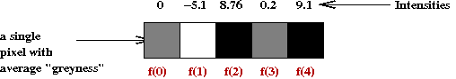
- Thus, a 2D array can be treated as a 2D array of intensities
  → an image!
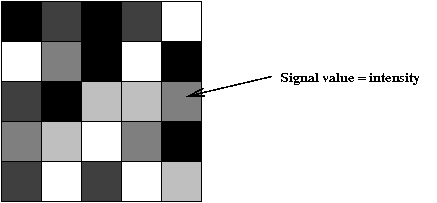
We'll assume square arrays of size $N \times N$.
→ It's easy to generalize to $M \times N$.
Let's use the notation $f(x,y)$ to denote the signal value in cell $(x,y)$, where $x$ and $y$ are integers.
Then, the input (signal) consists of:
- The number $N$.
- A collection of $N^2$ numbers $f(x,y)$ where $0 \leq x \leq N-1$ and $0 \leq y \leq N-1$.
- Alternatively, we can think of the input as $N^2$ complex numbers with the imaginary parts zero.
The output (spectrum) will be a 2D array of complex numbers $F(u,v)$.
The two dimensional DFT is defined as: $$ F(u,v) \eql \frac{1}{N^2} \sum_{x,y} f(x,y) e^{-2\pi i(ux+vy)/N} $$
Likewise, the inverse DFT is defined as: $$ f(x,y) \eql \sum_{u,v} F(u,v) e^{2\pi i(ux+vy)/N} $$
The FFT can also be generalized analogously, but is rather more complicated to describe.

In-Class Exercise 30: Compile and execute DemoDFT2D.java. You will also need Clickable2DGrid.java. The top two grids represent the signal's real (left) and imaginary (right) parts. The bottom two grids represent the spectrum.

Select the middle grid cell in the spectrum's real components and change this value to 100. Then, apply the inverse transform.

Click on "showValues" to examine the signal's values.

Change $N$ to 20 and repeat. Experiment with setting only one spectrum value to 100, but in different places.

The meaning of "frequency" in 2D:

In 1D, frequency is a way of measuring how the signal fluctuates.
In 2D, frequency measures fluctation of the signal spatially.
Thus, a single spectrum value corresponds to a checkboard pattern of some kind (depending on the frequency).
Just like the 1D case, the signal is an addition of the signals you get from individual frequencies.

What corresponds to removing high-frequencies in the 2D case?

We can also remove high frequencies and produced a modified signal image.
This is the basis of lossy image compression.
As it turns out, a DFT variant called the Discrete Cosine Transform, is more commonly used in image compression.

Summary and applications

Let's summarize what we've learned and point out some directions for future reading:

The sensation of sound arises from the eardrum reacting to fluctuations in air pressure
→ Constant pressure is silence.
Any analog sound can be represented as a function $f(t)$.
By Fourier's theorem, any function can be represented as a sum of sinusoids.
→ Any analog sound can be decomposed into a sum of sinusoids. $$ f(t) \eql a_0 \plss \sum_{k} a_k \sin(\frac{2\pi kt}{T}) \plss \sum_{k} b_k \cos(\frac{2\pi kt}{T}) $$
The Discrete Fourier Transform (DFT) takes a collection $M$ numbers and produces $M$ complex numbers.
- In the 1D case, $M=N$, the number of samples.
- In the 2D case, $M=N^2$, the number of samples.
The Fast Fourier Transform (FFT) is merely a faster ($O(N \log N)$ way of computing the DFT.
Digitized sound consists of sampling analog sound at fixed intervals.
The DFT applied to digitized sound extracts the frequency content provided the sampling was done at a high-enough frequency.
The DFT (really, the FFT) is one of the most useful and most used algorithms of all time.

Applications:

The general area of analyzing and manipulating signals is called signal processing.
Signal processing applications include:
- Filtering or removing certain frequencies
  → Think "equalizer" in an audio system.
- Noise removal (a particular kind of filtering)
  → For example, in radio communication.
- Smoothing
  → Improving the quality of sound.
Compression
→ Both MP3 and JPEG use DFT-like transforms.
One of the most spectacular applications of the DFT in history: Big Bang theory
- Big Bang theory predicts the existence of CMBR: cosmic microwave background radiation, in a particular frequency range.
- In the 1960's, Penzias and Wilson discovered and identified this radiation by separating out the frequency from radio signals.
- Later George Smoot and others confirmed this with detailed and more careful analysis, again using Fourier analysis to separate out the frequencies.
- This turned out to be a key supporting piece of evidence in Big Bang theory.
Perhaps surprisingly, Fourier analysis has been a key driver in the development of a great deal of modern math:
- A deeper, more abstract understanding of vector spaces and linear systems.
- Notions of limits and limits of functions (uniform convergence).
- Transform theory (and other types of transforms).