Two key chemicals in living things:
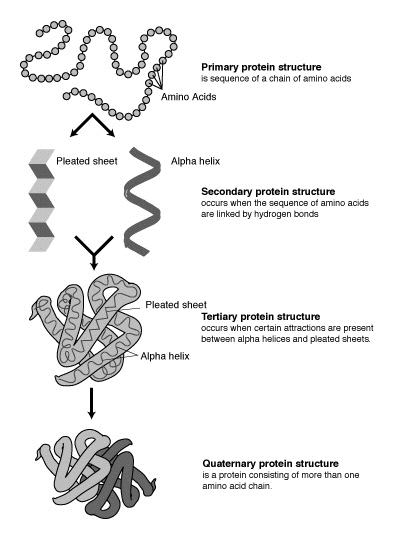
- Proteins:
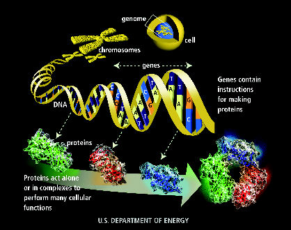
(Courtesy: Dept. of Energy)
- DNA:
Another view: two key languages:
- "Protein language"
- Protein = word
- Amino-acid = letter
- Alphabet = { A1, A2, ..., A20 }
(20 amino acids).
- "DNA language"
- DNA = sentence
- Base = letter
- Group-of-three-bases = word (called codon)
- multiple codons (protein encoder) = phrase
- Alphabet = { A, T, C, G }.
In-Class Exercise 12.1:
A single bit can encode two unique items (use "0" for one item, "1"
for the other item). Now, answer the following:
- How many unique items can k bits encode?
- How many unique items can a single letter in the alphabet
{ A, T, C, G } encode?
- How many unique items can be encoded with a k-letter word over the
alphabet { A, T, C, G }?
- What size word (i.e., what should k be) is enough to
encode 20 unique items?
What does DNA do?
- DNA's dual purpose:
- To encode proteins (build the creature).
- To replicate itself (propagate).
- Encoding proteins:
- 3-base substrings of DNA are used to encode (produce) amino
acids
⇒ a long sequence of DNA can encode a long sequence of
amino acids
⇒ a protein
- Recall: there are exactly 20 amino acids.
- Which 3-base combinations encode which amino acids?
Rules (the genetic code):
- DNA replication:
DNA replicates by a simple "photocopying process"
- A strand separates out:

- The strand creates its complement, drawing on available bases:

- The complement creates its complement:
12.2
DNA Alignment - A Problem in Computational Biology
In-Class Exercise 12.2:
Consider quantifying the distance between
strings. For example, "Bolt" is closer to "Bold" than
it is to "Bowl" or "Bot". What is a reasonable metric
and what are the distances for the above examples using
your metric?
Gene comparisons:
- Recall: a gene is a substring of DNA.
- Biologists often compare two genes from different animals to
see if they are "similar"
⇒ to help with gene identification.
- Example: Suppose the DNA sequence A T T T C G C C G T A C is the
"claw sharpness" gene in animal X.
⇒ can search for this gene in animal Y.
- Unfortunately, genes with identical function in different
animals are not identical.
- However, they are often similar, e.g.,
- Sometimes the similarity or "match" is more complex:
- By deliberately inserting spaces between the bases in one, a
better match can be found.
The alignment problem:
- Define scoring rules for evaluating a particular alignment:
- Perfectly matched letters get a high score.
- Matches between related letters get a modest score.
- Matches with gaps get a low score.
- The alignment problem: given two strings and the scoring
rules, find the optimal alignment.
- Problem components:
- An alphabet, e.g., { A, C, G, T }.
- Two input strings, e.g.,
- Match and gap scores, e.g.,
- Goal: find the alignment with the best (largest) value.
- Potential asymmetry:
- Some letter-alignments may be more favored.
- Some gap costs are different.
- Example:
- Example:
In-Class Exercise 12.3:
Use the above table to
compute the alignment scores (by hand) for the following alignment
of CGGAT and CGT:
      C G G A T
      C G T
Can you find a better alignment?
Key ideas in solution:
- First, the alignment problem can be expressed as a
graph problem:
- The diagonal edges correspond to character matches
(whether identical or not).
- Each down edge corresponds to a gap in string 2.
- Each across edge corresponds to a gap in string 1.
- Goal: find the longest (max value) path from top-left to bottom-right.
⇒ longest-path problem in DAG.
- Can be solved in O(mn) time (using topological sort)
(m = length of string1, n = length of string2).
- Suppose we label the vertices (i, j) where
i is the row, and j is the column.
- The best path to an intermediate node is via one of its
neighbors: NORTH, WEST or NORTHWEST.
- Dynamic programming approach:
- Building an actual graph (adjacency matrix etc) is unnecessary.
- Let Di,j
= value of best path to node (i,j) from (0, 0).
= score of optimal match of first i chars in string 1
to first j chars in string 2.
- Define (for clarity)
| Ci-1,j-1 |
= |
Di-1,j-1 + exact-match-score |
| Ci-1,j |
= |
Di-1,j + string1-gap-score |
| Ci,j-1 |
= |
Di,j-1 + string2-gap-score |
- Thus,
| Di,j |
= |
max (Ci-1,j-1, Ci-1,j, Ci,j-1) |
| |
= |
max (Di-1,j-1 + exact-match-score,
Di-1,j + string1-gap-score,
Di,j-1 + string2-gap-score) |
- Initial conditions:
- D0,0 = 0
- Di,0 = Di-1,0 + gap-score for
i-th char in string 1.
- D0,j = D0,j-1 + gap-score for
j-th char in string 2.
Implementation:
- Pseudocode:
Algorithm: align (s1, s2)
Input: string s1 of length m, string s2 of length n

1.    Initialize matrix D properly;

      // Build the matrix D row by row.
2.    for i=1 to m
3.        for j=1 to n
              // Initialize max to the first of the three terms (NORTH).
4.            max = D[i-1][j] + gapScore2 (s2[j-1])
              // See if the second term is larger (WEST).
5.            if max < D[i][j-1] + gapScore1 (s1[i-1])
6.                max = D[i][j-1] + gapScore1 (s2[i-1])
7.            endif
              // See if the third term is the largest (NORTHWEST).
8.            if max < D[i-1][j-1] + matchScore (s1[i-1], s2[j-1])
9.                max = D[i-1][j-1] + matchScore (s1[i-1], s2[j-1])
10.           endif
11.           D[i][j] = max
12.       endfor
13.   endfor

      // Return the optimal value in bottom-right corner.
14.   return D[m][n]

Output: value of optimal alignment
- Explanation:
- The 2D array D[i][j] stores the Di,j values.
- The method matchScore returns the value in matching
two characters.
- The method gapScore1 returns the value of matching a
particular character in string 1 with a gap.
(gapScore2 is similarly defined).
- Note: D[i][0] and
D[0][j] represent
initial conditions.
- Note: there is one more row than the length of string 1.
(likewise for string 2).
- Computing the actual alignment:
- A separate 2D array tracks which term contributed to the
maximum for each (i, j).
- After computing all of D, traceback and obtain path (alignment).
In-Class Exercise 12.4:
Download this template and
implement the above algorithm. Gap and match costs are given.
Analysis:
- The double for-loop tells the story: O(mn) to compute Dm,n.
- Note: computing the actual alignment requires tracing back:
O(m + n) time (length of a path).
- Space required: O(mn).
An improvement (in space):
- Genes are often longer than 10,000 bases (letters) long
⇒ space required is prohibitive.
- First, note that we only need successive rows in computing D
⇒ space requirement can be reduced to O(n).
- However, O(mn) space is still required to construct
the actual alignment.
- A different approach:
- Consider the "middle" character in string 1
⇒ the character at position m / 2.
- In the optimal alignment, this character will either align
with some j-th character in string 1, or a gap.
⇒ we can try all possible j values.
- To try these alignments, compute the m/2-th row (in
O(mn) time).
- Output the optimal alignment found.
- Recurse on either side of the optimal alignment.
- It is possible to show: O(mn) time and O(n) space.
Variations of the alignment problem:
- Alignment without end-gap penalty
⇒ do not add costs for gaps at ends.
- Substring alignment
⇒ find substrings that align.
- Length-based gap penalties
⇒ the longer a contiguous gap, the more the penalty.
- All have polynomial-time solutions.
12.3
Other problems in computational biology
The protein folding problem:
- Recall: a protein is a string of amino acids.
- A protein folds into its natural conformation
(shape)
⇒ The shape determines its function.
- Folded proteins are like 3-D jigsaw pieces
⇒ Two proteins interact by docking
- The protein folding problem:
given the 1-D sequence, determine the 3-D structure.
- To see why this is a hard problem, let's consider a
2D version of the problem:
- Folding occurs in the 2D plane:
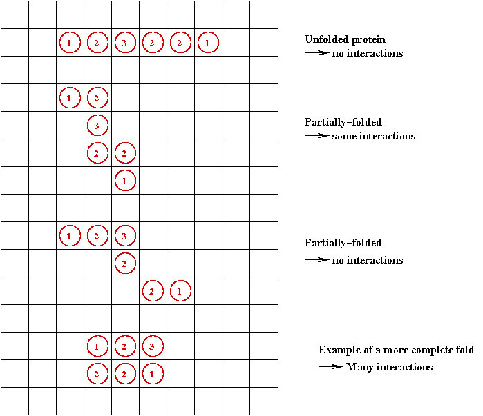
- Each potential fold has an energy "cost".
- Goal: find the minimal energy fold.
⇒
A combinatorial optimization problem.
- What parameters play into energy costs? Many physical
parameters, e.g.
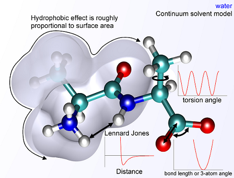
(Courtesy: wikicommons)
- In 3D with real proteins, the problem is much harder:
(Courtesy: wikicommons)
Other problems:
- Gene finding
⇒
Given a genome, identify genes within the genome.
- Phylogenetics and the tree of life.
⇒
Goal: build best possible tree.
- Pattern classification and microarrays
⇒
Given a DNA sample, classify the sample
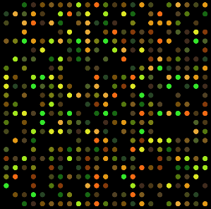
(Courtesy: wikicommons)
-
Biological networks
12.4
Cellular Automata and Von Neumann's Quandary
Cellular Automata:
- What is a cellular automaton?
- An infinite cellular space - usually a 2D grid:
- Set of states, e.g, S = { empty, A, B, C, D }.
- Initially each cell is in one of the states:
- System evolves in time-steps.
- At each step, "rules" are applied to generate the next state
for each cell, e.g.,
- State-transition rules:
- A neighborhood for each cell is defined, usually one of
- 4-neighborhood (N, S, E, W).
- 8-neighborhood (N, S, E, W, NE, NW, SE, SW).
- The next state of a cell depends on its current state and the
current state of its neighbors.
- All cells change state at the same time.
- The rules are sometimes called the "physics" of the system.
In-Class Exercise 12.5:
Search the web for applets that simulate the Game of Life and examine
what happens to the following patterns. Run each pattern for a few
time steps (generations).
- The Blinker.
- The Block.
- The Glider.
- The R-pentonimo.
The Game of Life:
- A cellular automaton with only two states: on and off.
- Devised in 1970 by John Horton Conway.
- Rules:
- Uses 8-neighborhood.
- Rule 1 (birth): if a cell has exactly 3 neighbors
"on", its next state is "on".
- Rule 2 (status-quo): if a cell has exactly 2
neighbors "on", its next state is its current state.
- Rule 3 (death): In all other cases, the next state is "off".
- A generalization: k-Game-of-Life
- Birth rule: if a cell has exactly k neighbors "on", its
next state is "on".
- Status quo rule: if a cell has exactly k-1 neighbors "on".
- Death rule: all other values.
- k = 3 in the Game-of-Life.
- Interesting observation:
- If k < 3: too much growth (chaos).
- If k > 3: too little growth (empty space).
- k = 3 is "optimal for life".
Von Neumann's quandary:
- Problem: to prove (mathematically) that self-reproduction is
possible.
- First attempt: the kinematic model (robots):
- Can a robot reproduce, i.e., assemble a copy of itself (that can later reproduce) from a blueprint?
- The blueprint problem: can a blueprint contain itself?
- Second attempt: cellular automaton.
- Trivial vs. non-trivial reproduction in cellular worlds:
- Trivial reproduction: the Blinker in the Game of Life.
- Von Neumann's criteria for non-trivial reproduction: a
cellular automaton that:
- Can embed a Universal Turing machine (i.e., can compute anything)
- Can embed a Universal Constructor (i.e., can build from a blueprint).
- Reproduce itself entirely, including blueprint.
- Von Neumann (with others) showed that it was possible: by constructing a
cellular automaton exhibiting non-trivial self-reproduction:
- 29 states per cell and 200,000 cells.
- The "creature" contained a "tape" with instructions (blueprint), and a
"constructor arm".
- Another part of the cellular creature contained a universal
Turing machine.
- Solution of the blueprint problem: the blueprint was
"photocopied" into the offspring.
- Reproduction occurs in two phases:
- Build the offspring by reading (interpreting) the blueprint.
- Copy over the blueprint into the offspring (without interpreting).
Other developments in cellular automata:
- The Game-of-Life can support computation (and it's believed) self-reproduction.
- Simpler non-trivial self-reproducing cellular automata have
been found
⇒ all use "blueprint copying".
(Example)
- Cellular automata have become a field of study with attempts
to build "metabolic" creatures (that grow, age, evolve etc).
Intriguing questions and comparison between cellular automata and
our "wet" world:
- Question: Does the physics/chemistry support
"self-reproducing life"?
| Cellular world |
Yes.
e.g, Von Neumann's example. |
| Wet World |
Yes. |
- Question: Does the physics also support trivial reproduction?
| Cellular world |
Yes.
Game-of-Life's Blinker |
| Wet World |
Yes.
Crystalline growth. |
- Question: Does non-trivial reproduction use the
2-step blueprint model?
| Cellular world |
Yes.
All examples |
| Wet World |
Yes.
DNA replication and interpretation. |
- Question: Is evolution supported?
| Cellular world |
Yes.
In some models. |
| Wet World |
Yes.
|
- Question: Is spontaneous occurrence of "life" possible?
| Cellular world |
Not known. |
| Wet World |
Current belief: Yes. |
- Question: Is uncontrolled chaotic growth ("grey goo") possible?
| Cellular world |
Yes.
Game-of-Life's R-pentonimo |
| Wet World |
? |
- Question: Do the elements of self-reproduction also
support computation?
| Cellular world |
Yes.
Many examples |
| Wet World |
Yes.
(next section) |
12.5
Computing with DNA
Yes, with actual DNA.
Key ideas:
- We will use chemical reactions with DNA to solve the
Restricted Hamiltonian Path problem
⇒ exploit the massive parallelism with millions of DNA molecules.
- The Restricted Hamiltonian Path problem (directed graph version):
- Given a directed graph and two vertices s and d,
find a path between s and d that visits each vertex
exactly once.
- Result: Restricted Hamiltonian Path problem is NP-complete.
- Note: for an n-vertex graph, the path is of length n.
- Overview of process:
- Represent vertices using strings of DNA bases.
- Represent edges using combinations of vertex-strings.
- Use gel-electrophoresis to extract DNA with correct length.
- Use filtering process in many steps to separate out paths
with all vertices.
⇒ solution (no pun intended) to Hamiltonian path problem.
In-Class Exercise 12.6:
Why is the Restricted Hamiltonian Path problem NP-complete (given that
the regular Hamiltonian Path problem is NP-complete)?
Details:
- Step 1 (on paper): associate unique DNA substrings with
vertices, e.g.
- In the above example, an 8-base string represents a vertex.
- In practice, a larger number is required to help separate out
different-length paths.
- Step 2 (on paper): associate unique DNA substrings with
edges, based on substrings for vertices:
- For edge ( v1, v2) join the
latter half of v1's string with the
first half of v2's string.
- Step 3 (on paper): identify the complementary strings for
the vertices, e.g.,
- Step 4 (on paper): create unique "start" and "stop" DNA
strings for vertices s and d.
- The "start" string represents an artifical edge between
"start" and s.
- The "end" string represents an artifical edge between
d and "end".
- Step 5 (lab): synthesize all of the above DNA material
(substrings) separately (one beaker corresponding to each different string).
- Step 6 (lab): mix all the edges and complementary vertices:
- The complementary vertices will, lego-like, bind edges in sequence.
- This will produce all possible paths in the graph, including
invalid ones (without "start" and "end").
- Step 6 (lab): extract all paths beginning with "start" and
ending with "end".
⇒ use (wet lab) PCR technique
- Step 7 (lab): separate out the DNA with the correct length
(exactly n substrings)
⇒ use gel-electrophoresis.
- Note: this will result in paths of exactly length n.
- However, it will also contain paths with repetitions.
- Step 8 (lab):
- Filter out all paths that don't contain the string for v1
⇒ use v'1 (complement) to bind.
- This leaves all paths containing v1.
- Next, filter out all paths that don't contain v2.
- ... repeat the above for all vertices in turn ... (a for-loop!)
- What remains: the DNA representation of all paths of length
n that contain all vertices
⇒ Hamiltonian paths!
Summary:
- The purpose was to show that DNA and chemical processes can "compute".
- Potential efficiency: chemical reactions occur in parallel.
- It is not yet a practical method:
- Problems need to be carefully coded.
- Encoding takes time.
- Macro-scale experimentation results in errors
⇒ (fraction of a teaspoonful required for 7-vertex graph).
- Related work:
- Using DNA for building "wetware" (gates, flip-flops).
- Using proteins for computation.
- Self-assembling nanoparticles.
12.6
Genetic Algorithms and Combinatorial Optimization Problems
Key ideas:
- Use evolution as a metaphor for "winnowing" solutions.
- Outline (for TSP):
- Each candidate TSP tour is a "genome" (animal).
- Start with a large number of potential solutions (initial population).
- At each step generate a new population:
- Use mutation to "explore"
- Use mating to preserve "good characteristics".
- Weak (high-cost) solutions "die".
- Strong (low-cost) solutions "survive".
- Eventually, optimal solution should dominate population.
Details: (TSP example)
- Input: the n TSP points.
- Associate tour with genome.
- A genome's fitness is the tour's length.
(shorter the better).
- Step 1: create an initial population of m random tours
(.e.g, m = 1000).
(They don't have to be unique).
- Step 2: Compute the "fitness" value of each genome (tour).
Example with four 5-city tours:
| ID |
Genome
(tour) |
Fitness
(inverse tour length) |
Fraction of
total (PDF) |
| 1 |
0-1-2-3-4 |
27.5 |
0.31 |
| 2 |
4-0-1-3-2 |
12.95 |
0.15 |
| 3 |
0-2-1-3-4 |
9.3 |
0.11 |
| 4 |
2-4-3-0-1 |
36.0 |
0.42 |
|
|
87.75
(total) |
1.00
(total) |
- Step 3: compute the population PDF (Probability Distribution
Function)
⇒ fraction based on fitness.
- Compute the total fitness (sum of tour costs).
- Compute what fraction of the total each fitness value amounts to.
- The fractions are the PDF.
- Step 4: generate a new population drawing from the PDF
⇒ about 31% (on average) of the new population will contain
genome 1 and 11% will contain genome 3.
- Step 5: Apply crossover rules (mating):
- The crossover-fraction is an algorithm parameter,
e.g., crossover-fraction = 0.3
⇒ 30% of genome-pairs will engage in crossover.
- Select a random 30% of pairs randomly (assuming
crossover-fraction = 30).
- Apply a crossover rule to each such pair: exchange parts of
genomes between the pair.
- Step 6: Apply mutation
- mutation-fraction is an algorithm parameter.
- mutation-fraction = fraction of genomes to mutate
(e.g., 0.05)
- Select 5% of the genomes (randomly) to mutate.
- Apply mutation to each (make a slight adjustment in the tour).
- Repeat steps 2-6 until fitness values converge
⇒ population is dominated by high-fitness genomes (tours).
Crossover and mutation in TSP:
- How do we "mate" two TSP tours?
- Take the first part (about half) of Tour 1.
- Take the remaining points in the order these points are found
in Tour 2.
- How do we mutate a TSP tour?
⇒ swap 2 points
In-Class Exercise 12.7:
Consider a 5-point Euclidean traveling salesman problem
with the following inter-point distances:
| | 1 |
2 | 3 | 4 |
| 0 | 5.0 | 3.0 | 4.2 | 3.0 |
| 1 | | 4.0 | 3.2 | 3.2 |
| 2 | | | 1.4 | 4.3 |
| 3 | | | | 4.6 |
Write down the default starting tour 0 1 2 3
4 and evaluate its fitness.
Start with a population of 4 tours: the default tour above
and 3 other randomly created tours.
Then, repeat the following three times:
- Make a random mutation. Use some physical source of randomness.
- For 2 of the tours, find a way "mate" them. For a 3rd tour,
create a random mutation. Leave the 4th tour as is.
- Now you have 4 new tours. Evaluate their fitness, and
change the population to feature only the two best tours.
What is the final best tour and its cost?
Summary:
- Advantages of genetic algorithms:
- Genetic algorithms are easy to implement.
- Like simulated annealing, the problem-specific part can be
separated out from the generic algorithm.
- If re-arrangements in fact do impact the solution, genetic
algorithms have a reasonable chance of finding a good solution.
- By its nature genetic algorithms try many initial solutions
(simultaneously)
⇒ simulated annealing needs to be re-run with different
starting solutions.
- Disadvantages:
- Genetic algorithms are slow.
- It's hard to define meaningful crossovers and mutations for
some problems.
- It requires some experimentation to get it working.
⇒ it's easier to automate this part in simulated annealing.
- Generally, simulated annealing (with appropriate
modification) is thought to be a better option.
- Warning:
- Its biological origins do not give it any special advantage
⇒ beware of its mystical appeal!
12.7
Other Biological Metaphors in Algorithms
Neural networks:
- Simplified neuron architecture:
- Artificial neuron:
- Structure:
- Rule: Neuron fires if X1 + X2 +
X3 > T.
- A simple application to pattern recognition:
- McCulloch-Pitt neuron model:
- Structure:
- Inputs: X1, X2, ..., Xn
- An "importance" weight Wi is associated with
each input i.
- Neuron has output only if W1X1
+ ... + WnXn > T.
- Networks of neurons:
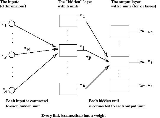
- Neural networks are used to approximate unknown functions.
- Key ideas:
- Each network has a set of parameters (neuron weights).
- Use a "training set" of samples from unknown function to set parameters.
- Once parameters are set, the function is approximated.
Other biological metaphors:
- Ant-colony optimization
- Evolutionary computation