Before describing what "NP-complete" means, we'll take a look at
some well-known problems.
Clique:
- What is a clique?
- In a graph, a clique is a subset of vertices with the property: there's
an edge between every pair of vertices
- Example:
- Optimization version:
Given a graph G=(V,E) find the
largest-size clique in the graph.
- Decision version:
Given a graph G=(V,E) and a number K, is there
a clique of size at least K?
- Application: finding complete sub-graphs (which itself has applications).
In-Class Exercise 11.2:
Draw an 8-vertex graph such that every vertex is in some clique of
size 3.
Vertex cover
- What is a vertex cover?
- In a graph, it's a subset of vertices such that every edge is
incident to at least one of these vertices.
- Example:
- Optimization version:
Given a graph G=(V,E) find the smallest-size vertex cover in the graph.
- Decision version:
Given a graph G=(V,E) and a number M is there a vertex cover
of size at most M?
- Application: place mailboxes on street-corners so that
every street is covered.
In-Class Exercise 11.3:
Draw an 8-vertex graph whose smallest vertex cover is of size 2.
Satisfiability (SAT)
- First, consider boolean expressions:
- Suppose x1, x2, ...,
xn are boolean variables.
- Boolean operators: AND, OR, NOT.
- Example boolean expression:
(x1 x2) + (x'2 x3)
+ (x2 x3x'4)
- Satisfiable expressions:
- A boolean expression is satisfiable if we can assign
true/false values to the variables to make the whole expression true.
- Example:
(x1 x2) + (x'2 x3)
+ (x2 x3x'4)
Setting x1 = x2 = x3 =
T makes the expression true.
- Conjunctive form:
- Every boolean expression can be converted into an equivalent
Conjunctive-Normal-Form (CNF):
- CNF: AND'ed sub-expressions that have only OR's and NOT's.
(x1 + x2 + x'3) (x'2+ x3)
(x'2 + x3 + x'4 + x5)
- Problem: given a CNF expression with n variables, is
it satisfiable?
- Note: decision and optimization version are the same in this problem.
- Variations:
- k-SAT: when the conjuncts are limited to k terms.
- 3-SAT: when the conjuncts are limited to 3
terms, e.g.,
(x1 + x2 + x'3) (x'2+ x3)
(x'2 + x'4 + x5)
- Applications: removal of dead-code, evaluation of circuits.
In-Class Exercise 11.4:
Is the expression
(x1 + x2) (x'1 + x'2+ x'3)
(x3 + x2 + x'4)
satisfiable?
Other problems (optimization versions briefly described):
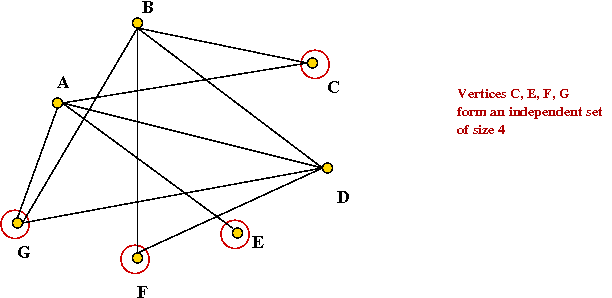
- Independent set: Given a graph, find the largest subset
of vertices such that no two vertices in the subset have an edge
between them.
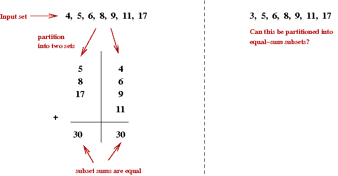
- Partition: Given items with sizes
s1, s2, ..., sn, is there
a partition of the items into two subsets of equal (total) size?
- Knapsack: Given a knapsack of size K, items with sizes
s1, s2, ..., sn and values
v1, v2, ..., vn,
which subset of items will fit into the knapsack and provide
maximum value?
- Multiprocessor scheduling: given M processors
and tasks with execution times s1, s2, ...,
sn, partition the tasks among the processors to
minimize overall completion time.
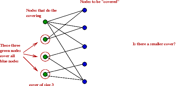
- Set cover: Given a collection of sets
S1, S2, ..., Sn
what is the minimal set of elements such that every set in the
collection has at least one element in the minimal set?
11.3
Transforming an Instance of one Problem into an Instance of Another Problem
Consider this unusual approach to solving a problem:
- Suppose we've written code to find the max of an array of
int's:
    Algorithm: max (A)
    Input: An array of int's A
        // ... find the max value in A and return it ...
- Now consider this:
    Algorithm: min (A)
    Input: An array of int's A
        // ... find the min value in A and return it ...
        for i=0 ...
            B[i] = - A[i]
        endfor
        m = max (B)
        return -m
- Notice the strange way of "solving" a different problem:
- We have an algorithm for problem X.
- We have a new problem Y.
- Transform the data, feed it to the algorithm for X
- Interpret the result as a solution to Y.
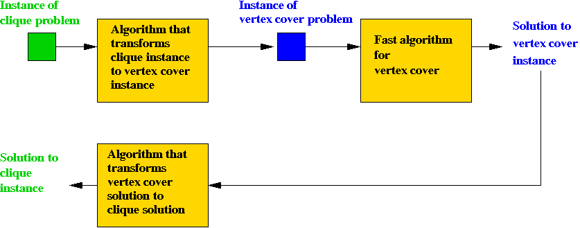
Now let's apply this to combinatorial optimization problems:
Example: transforming clique to vertex cover:
- Suppose we are given an instance of the clique problem,
G = (V, E).
⇒ Recall: goal is to find largest clique.
- Example:
- Define G', the complement of G as follows:
- G' has the same vertex set V of G.
- For every two vertices, u, v not connected in
G, place an edge in G'.
- Claim: if G' has a vertex cover of size k then
G has a clique of size n - k:
- Performing the transformation has two parts:
- Transforming G to G':
- Processes each pair of vertices once
⇒ O(n2) time to transform an instance of
clique into an instance of vertex cover.
- Transform vertex cover solution to clique
solution:
- Build clique graph
⇒ O(n2) time (worst-case).
Thus, both transformations take polynomial-time.
Decision version:
- Decision version of clique:
Is there a clique of size at least k?
- Decision version of vertex cover:
Is there a vertex cover of size at most m?
- What we have shown:
size-(n-k) vertex-cover in G' ⇔
size-k clique in G.
- Thus, we can create a solution for the decision version of clique:
Time taken:
- Suppose the vertex-cover algorithm takes time P1(n).
- Next, suppose the transformation takes time P2(n).
- We have a clique algorithm that takes time
P1(n) + P2(n), still a polynomial.
Some other known transformations:
- Satisfiability (3-SAT) to clique.
⇒ suppose the transformation takes time P3(n).
⇒ we can build an algorithm for 3-SAT:
- Hamiltonian-tour to 3-SAT.
⇒ suppose the transformation takes time P4(n).
⇒ we can build an algorithm for Hamiltonian-tour
In-Class Exercise 11.5:
Consider the following problem:
- There are n items with weights
w1, w2, ..., wn respectively.
- There are K people who are to carry these items on
a trip.
- We would like to distribute the weights as evenly as possible.
Let us call this the weight distribution problem.
Answer the following questions:
- Formulate the problem as a combinatorial optimization problem.
- State the decision version of the problem.
- Show that the decision version of Bin-Packing Problem (BPP) can be
transformed into the decision version of this problem.
11.4
The Theory of NP-Completeness (Abridged)
NP problems:
- NP problems are those decision problems whose candidate solutions
can be verified in polynomial-time.
- Example: TSP
- Recall decision version: is there a tour of length at most L?
- Candidate solution is a tour.
- Given a particular tour, how long does it take to check whether its length is
at most L?
⇒ O(n) time.
⇒ TSP is an NP-problem.
- Example: BPP
- Decision version: can the given items fit into at most K bins?
- Candidate solution is an assignment.
- How long does it take to check whether the assignment uses at
most K bins?
⇒ O(n2) (worst-case, given assignment matrix).
⇒ BPP is an NP-problem.
- Most combinatorial problems are NP problems.
- Note: NP = "Nondeterministic Polynomial-time" (theoretical
reason for this name).
- Formal way of stating a problem is an NP-problem: the
problem is in the language NP.
First fundamental result:
- If you can solve k-SAT in polynomial time, you can solve any
problem in NP in polynomial time.
⇒ Every NP-problem is no harder than k-SAT
- Proof is elaborate and uses a construction with Turing machines.
- Landmark result proved by Steve Cook in 1972.
Second fundamental result(s):
- Many combinatorial optimization problems can be transformed
into another combinatorial optimization problem in polynomial-time.
⇒ These problems are "equally hard" (to within a polynomial)
- We have already seen examples of this transformation.
- First few landmark results proved by Richard Karp in 1973.
Thousands of such transformations since then.
NP-Completeness:
- A problem is NP-complete if:
- It is an NP-problem.
⇒ The problem is no harder than k-SAT
- Some other existing NP-complete problem can be transformed
into it in polynomial-time.
⇒ It is at least as hard as other NP-complete problems (including k-SAT).
Major implication of the two results:
- If you can solve ANY ONE NP-complete problem in polynomial-time
you can solve EVERY ONE of them in polynomial-time.
- Thus, they are all of (polynomially) equivalent complexity.
- The classes P and NP:
- Let P be the set of problems solvable in polynomial-time
(e.g., MST is in P).
- NP is the set of problems described above.
- If a polynomial-time algorithm is found for any NP-complete
problem, then P = NP.
- The most famous
outstanding problem in computer science: is P = NP?
- Most experts believe P is not equal to NP.
- Note: just about every interesting combinatorial problem
turns out to be NP-complete (thousands of them).
What to do?
- Approach 1: solve problems approximately
⇒ fast algorithm, possibly non-optimal solution.
- Approach 2: solve problems by exhaustive search
⇒ optimal solution, but really slow algorithm.
11.5
Approximate Solutions
Key ideas in approximation:
- Devise algorithm to make "intelligent guesses" and arrive at a
"good" (but not optimal) solution.
- Evaluating an algorithm: how close to optimal are its solutions?
- Theoretical analysis: prove a bound (e.g., no worse than
twice optimal).
- Experimental: evaluate algorithm using randomly-generated data.
- Typical theoretical analysis:
- Let C* be the optimal cost.
- Let CA be the cost of solution produced by
algorithm A.
⇒ CA \(\geq\) C*
- Question: how far off is CA from C* ?
- Try to prove: CA < k C* (for small k).
- TSP example: we will show that CA < 2 C*.
⇒ No worse than twice optimal
An approximation algorithm for (Euclidean) TSP:
- Euclidean TSP satisfies the triangle inequality:
- Consider any three points p1, p2
and p3
- Then, dist(p1, p2) ≤
dist(p1, p3) + dist(p3, p2).
- The algorithm:
- First find the minimum spanning tree (using any MST
algorithm).
- Pick any vertex to be the root of the tree.
- Traverse the tree in pre-order.
- Return the order of vertices visited in pre-order.
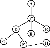
In-Class Exercise 11.6:
Write pseudocode for generating a pre-order. What is
the pre-order for this tree (starting at A)?
- Example:
- Consider these 7 points:
- A minimum-spanning tree:
- Pick vertex A as the root:
- Traverse in pre-order:
- Tour:
- Claim: the tour's length is no worse than twice the optimal
tour's length.
An approximation algorithm for BPP: First-Fit
- The algorithm:
- Consider items in the order given (i.e., arbitrary order).
- For each item in order:
- Scan current bins in order to see if item fits anywhere.
- If not, place item in new bin.
- Claim: number of bins is no more than twice the optimal number
of bins.
- Let B = bin size.
- Let S = sum of item sizes.
- Let b = the number bins used by the algorithm.
- Let b* = optimal number of bins.
- Algorithm cannot leave more than two bins only half-full:
- Thus, the most bins are used when all are just over half-full.
⇒ b ≤ S / (B / 2) = 2S / B.
- Optimal solution cannot be better than fractional optimal
solution S / B.
- Thus, b ≤ 2 b*.
- It is possible (lengthy proof) to show:
- b < 1.7 b* + 2 (no more than 70% worse).
- There are cases when b > 1.7 b* - 1 (at least 70% worse).
⇒ b < 1.7b* is the best FF can do.
- Decreasing First-Fit algorithm: sort in decreasing order
first and then apply FF.
- Best known result: b < 1.22 b* (difficult proof).
The world of approximation:
- For many NP-complete problems, there are results on approximation algorithms.
- Theoretical results:
- Proofs that an algorithm is "close" to optimal.
- Proofs that an algorithm is definitely worse than optimal.
- Sharper bounds for algorithms.
- Experimental results:
- Comparisons with large "real" data sets
(e.g, TSP on state-capitals in the U.S.).
- Comparisons using randomly-generated data.
- Approximation algorithms for polynomially-solvable problems:
- Sometimes the polynomial-time solution takes too long for
large n (e.g, n3)
⇒ a faster approximation-algorithm may be desirable.
Known approximation results for TSP:
- 1992: Unless P=NP, there exists ε>0 such that
no polynomial-time TSP heuristic can guarantee
CH/C* ≤ 1+ε
for all instances satisfying the triangle inequality.
- 1998:
For Euclidean TSP, there is an algorithm that is polyomial for fixed
ε>0 such that
CH/C* ≤ 1+ε
- 2006:
→
Largest problem solved optimally: 85,900-city problem.
- 2009: Best practical heuristic
→
1,904,711-city problem solved within 0.056% of optimal
In-Class Exercise 11.7:
Download this template as well
as UniformRandom, and
implement the First-fit and Decreasing-First-Fit algorithms for Bin Packing.
11.6
Exhaustive Search
Key ideas:
- To find the optimal solution of an NP-complete problem,
exhaustive search can be used
⇒ try every possible "state" in the state-space.
- Exhaustive search is feasible for small problem sizes.
(e.g., n < 15)
- However, there are ways of cleverly avoiding some solutions
by pruning the search
⇒ can solve larger problems (typically n < 30).
- Two types of search:
- Enumeration: enumerate all possibilities one by one
and track the "best".
- Advantages:
Easy to implement, does not require understanding the problem in detail.
- Disadvantages:
Takes no advantage of problem structure.
- Constructive state-space search:
- Builds up solutions in pieces.
- Conceptually, full-solutions are leaves of a tree.
- TSP Example: build tours from partial-tours.
- Two flavors: Backtracking and Branch-and-bound.
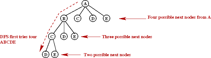
- Backtracking: roughly, a depth-first search of tree.
- Branch-and-bound: roughly, a breadth-first search
of tree.
- Both can be speeded up with pruning (avoiding
unnecessary exploration).
- Backtracking example with TSP on five vertices:
11.7
Exhaustive Enumeration
We will consider methods for:
Note: we want methods with small memory requirements
⇒ cannot store all combinations or permutations.
⇒ must be able to "generate" next combination/permutation
from most recent one.
11.8
Generating All Possible Subsets
Key ideas:
- Suppose n = number of elements in set.
- Bit-pattern equivalence:
- Example: consider the subset { 1, 3, 4 } of { 1, 2, 3, 4, 5 }
- Use the bitstring "1 0 1 1 0" to represent this subset.
- The i-th bit is "1" if the i-th element is in the particular subset.
- Given a bit-pattern, it's easy to produce the equivalent
subset
⇒ extract those elements whose bit is "1".
- Thus, "generating all subsets" is equivalent to "generating
all bit patterns".
- Key observations:
- There are 2n bit patterns.
- If the bit-patterns are treated as binary numbers
⇒ all we have to do is enumerate the binary numbers 0, 1,
..., 2n-1
- For each such bit-pattern produced, create the corresponding subset.
- Example: if S = {1, 2, 3}
- "0 0 0" = Empty set.
- "0 0 1" = { 3 }
- "0 1 0" = { 2 }
- "0 1 1" = { 2, 3 }
- "1 0 0" = { 1 }
- "1 0 1" = { 1, 3 }
- "1 1 0" = { 1, 2 }
- "1 1 1" = { 1, 2, 3 }
In-Class Exercise 11.9:
What is the next subset for the following subset (of a 5-element set):
10111?
Implementation
- We will use a boolean array called member
⇒ member[i]=true if element i is in the current set.
- We will write code to generate one element from the previous one:
- We will use the natural order of binary numbers.
- Example: if current subset is "1 0 1", the next subset is "1 1 0".
⇒ add "1" to current number to get the next.
- We will write:
- A method getFirstSubset to initialize and create the first subset.
- A method getNextSubset to be called for each
successive subset.
- Pseudocode:
Algorithm: getFirstSubset (N)
Input: the size of the set

1.    member = create boolean array of size N;
      // First subset corresponds to "0" in binary.
2.    for each i, member[i] = false
3.    return member

Output: first subset - the empty set.
Algorithm: getNextSubset (member)
Input: current subset, represented by boolean array member
      // Start at the rightmost bit.
1.    i = N-1

      // Binary addition: as long as there are 1's, flip them.
2.    while i >= 0 and member[i] = true
3.      member[i] = false
4.      i = i -1
5.    endwhile

      // Did we run past the beginning of the array?
6.    if i < 0
        // Yes, so all were 1's and we're done with generation.
7.      return null
8.    else
        // No, so we found a zero where the carry-over from binary
        // addition finally stops.
9.      member[i] = true
9.      return member
10.   endif

Output: return new subset in which member[i]=true if i is in the subset.
In-Class Exercise 11.10:
This exercise is optional.
Download this template and
try implementing the above pseudocode.
11.9
Generating All Possible Combinations
Key ideas
- Goal: generate all k-size subsets from the integers 0, ..., n-1
- We will use the bitstring idea from above
⇒ every bitstring will have exactly k one's.
In-Class Exercise 11.11:
How many size-3 subsets does a 5-element set have?
Write down the corresponding bit patterns.
Implementation
- Data structures:
- member - a boolean array where member[i] = true if
element i is in the current set.
- position - an integer array where
positions[i] = 1 if there is a 1 in the i-th position.
- The code will be spread over three methods:
- translatePositionsToSet
- given a particular arrangement of 1's, create the actual subset.
- getFirstCombination - initialize and return first combination.
- getNextCombination - generate next combination by
shifting 1's.
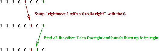
- High-level pseudocode:
Algorithm: getNextCombination ()
Input: current combination.
1.    r = position of rightmost 1 with a 0 to it's right;
2.    swap (r, r+1)
3.    bunch up all 1's in positions r+2,...,n-1 to the right of r+1
4.    return new combination
- Detailed pseudocode:
Algorithm: translatePositionsToSet (positions)
Input: an array with k 1's.
1.    Set member array so member[i]=true when position[i]=1
2.    return member
Output: member array
Algorithm: getFirstCombination (N, k)
Input: integers N and k

      // Create space for arrays.
1.    Create new arrays member and position;

      // Bunch up the k 1's to the left.
2.    for i=0 to k-1: positions[i] = 1

      // Return the corresponding subset.
3.    member = translatePositionsToSet (positions)
4.    return member

Output: initial set elements via the membership boolean array.
Algorithm: getNextCombination (member)
Input: current combination. Also, current positions array is accessible.

     // The trivial case:
1.   if N=1
2.     return null
3.   endif

     // Find the rightmost 1 that is followed by a 0.
4.   r = position of rightmost 1 with a 0 to the right of it;

     // If we couldn't find one, all are bunched up to the right, so we're done.
5.   if r < 0
6.     return null
7.   endif

     // Otherwise, we've found a 1. Next, count the 1's to the right of it.
8.   count = find all 1's to the right of position r;

     // Switch the 1 with the zero to its right.
9.   swap (r, r+1)

     // Now bunch up the 1's to the right of our special 1.
10.  for j=1 to count
11.    positions[r+1+j] = 1
12.  endfor

     // The remaining are all 0's.
13.  Set positions[j] = 0, for j > r+1+count

     // This creates the new subset to return.
14.  member = translatePositionsToSet (positions)

15.  return member

Output: member array for next combination
- A complete example with N=5 and k=3 (two steps shown per combination):
    1 1 1 0 0       Rightmost 1-followed-by-0 found at position 2

    1 1 0 1 0       Moved the 1 found rightwards and bunched up the 1's to the right


    1 1 0 1 0       Rightmost 1-followed-by-0 found at position 3

    1 1 0 0 1       Moved the 1 found rightwards and bunched up the 1's to the right


    1 1 0 0 1       Rightmost 1-followed-by-0 found at position 1

    1 0 1 1 0       Moved the 1 found rightwards and bunched up the 1's to the right


    1 0 1 1 0       Rightmost 1-followed-by-0 found at position 3

    1 0 1 0 1       Moved the 1 found rightwards and bunched up the 1's to the right


    1 0 1 0 1       Rightmost 1-followed-by-0 found at position 2

    1 0 0 1 1       Moved the 1 found rightwards and bunched up the 1's to the right


    1 0 0 1 1       Rightmost 1-followed-by-0 found at position 0

    0 1 1 1 0       Moved the 1 found rightwards and bunched up the 1's to the right


    0 1 1 1 0       Rightmost 1-followed-by-0 found at position 3

    0 1 1 0 1       Moved the 1 found rightwards and bunched up the 1's to the right


    0 1 1 0 1       Rightmost 1-followed-by-0 found at position 2

    0 1 0 1 1       Moved the 1 found rightwards and bunched up the 1's to the right


    0 1 0 1 1       Rightmost 1-followed-by-0 found at position 1

    0 0 1 1 1       Moved the 1 found rightwards and bunched up the 1's to the right
In-Class Exercise 11.12:
This exercise is optional.
Download this template and
try implementing the above pseudocode for generating combinations.
11.10*
Generating All Possible Permutations
Key ideas
Implementation
- High-level pseudocode:
Algorithm: getNextPermutation ()
Input: current permutation.
1.    Find highest-numbered mobile element.
2.    Move this one step in its current direction.
3.    Reverse its direction and the direction of all higher-numbered elements.
4.    return new permutation.
- Data structures:
- permutation - an integer array where permutation[j] = i if
element i is in the j-th position of a permutation.
- pointsLeft - a boolean array where
pointsLeft[i] = true if element i points left (it points
right, otherwise).
- The code will be spread over two methods:
- getFirstPermutation - initialize and return first permutation.
- getNextPermutation - generate next permutation from
the current one.
- Pseudocode:
Algorithm: getFirstPermutation (N)
Input: the number of items N (Thus, the integers 0, ..., n-1).

     // Create space and initialize.
1.   Create arrays permutation and pointsLeft.
2.   for each i, permutation[i] = i
3.   for each i, pointsLeft[i] = true
4.   return permutation

Output: the first permutation 0 1 ... (n-1)
Algorithm: getNextPermutation (permutation)
Input: the current permutation, where permutation[j] = i means
       number i is the j-th position in the permutation.

      // Locate the largest mobile element in the current permutation.
      // Recall: an element can move only in its current direction and
      //         if there's a smaller element next to it in that direction.
1.    m = position of largest mobile element in permutation array;

      // Only the permutation (n-1) ... 2 1 has no mobile elements.
2.    if no mobile elements
3.      return null

      // Move the largest mobile element in its current direction.
      // Mustn't forget to swap in both arrays.
4.    if pointsLeft[m]
5.      swap (permutation, m, m-1)
6.      swap (pointsLeft, m, m-1)
7.    else
8.      swap (permutation, m, m+1)
9.      swap (pointsLeft, m, m+1)
10.   endif

      // Change the direction of all elements larger than the one just moved.
11.   largestMobileValue = permutation[m]
12.   Switch directions of all elements larger than largestMobileValue;

      // Return newly generated permutation.
13.   return permutation
In-Class Exercise 11.13:
This exercise is optional.
Download this template and
try implementing the above pseudocode for generating permutations.