Module 7: Analysis of Algorithm Performance

Linked list vs. Array list

Recall the three basic operations implemented earlier for a linked list:

insert: inserting or "adding" a new element to the list.

search: to see if a given element exists in the list.

get(i): to retrieve the i-th element in the list.

The structure of the linked list class looked like this:

public class OurLinkedList {

    // ... variable declarations ...

    public void add (Integer K)              // Insert operation.
    {
        // ...
    }

    public boolean contains (Integer K)      // Search operation.
    {
        // ...
    }

    public Integer get (int i)               // get() operation.
    {
        // ...
    }

}

The other data structure we created for this purpose was the array-list, with exactly the same operations:

public class OurArrayList {

    // ...

    public void add (Integer K)              // Insert operation.
    {
        // ...
    }

    public boolean contains (Integer K)      // Search operation.
    {
        // ...
    }

    public Integer get (int i)               // get() operation.
    {
        // ...
    }

}

Let us next compare the performance of these two data structures for each of these operations:

We'll use a list of integers in our example.
For insert, we will start with an empty list and add a large number of integers (elements).
For search, we will perform a number of searches in a large list.
For get(), we will randomly generate positions in the list from which to retrieve an element.

Here is some of code:

public class ListComparison {

    public static void main (String[] argv)
    {
        // Use a 10,000-insertions (repeat for 1000 samples).
	testInsert (1000, 10000);

        // Use a list with 100000 elements (repeat for 1000 samples).
	testSearch (1000, 100000);

        // Use a list with 100000 elements (repeat for 1000 samples).
	testGet (1000, 100000);
    }


    static void testInsert (int numTrials, int numElements)
    {
        // Evaluate the "insert" operation in a linked-list.

        // Repeat for given number of trials.
	double total = 0;
	for (int k=0; k < numTrials; k++) {

	    long startTime = System.currentTimeMillis();

	    // Make a list and add numElements to it.
	    OurLinkedList list = new OurLinkedList ();
	    for (int i=0; i < numElements; i++) {
		list.add (i);
	    }

	    long timeTaken = System.currentTimeMillis() - startTime;
	    total += timeTaken;

	}

        // This is the average insert time.
	double avg = total / numTrials;
	System.out.println ("Average insert time for linked list: " + avg);


        // Now repeat for an array list.

	total = 0;
	for (int k=0; k < numTrials; k++) {
	    long startTime = System.currentTimeMillis();
	    // Make a list and add numElements to it.
	    OurArrayList list = new OurArrayList ();
	    for (int i=0; i < numElements; i++) {
		list.add (i);
	    }
	    long timeTaken = System.currentTimeMillis() - startTime;
	    total += timeTaken;
	}

        // Average for the array list.
	avg = total / numTrials;
	System.out.println ("Average insert time for array list: " + avg);
    }



    static void testSearch (int numTrials, int numElements)
    {
        // ... similar ...
    }


    static void testGet (int numTrials, int numElements)
    {
        // ... similar ...
    }

}

Note:

We've called our programs OurLinkedList and OurArrayList to distinguish them from the ones in the Java library called LinkedList and ArrayList.
The unit of time above is in milliseconds.

This is a sample execution on three different platforms:

Operation	2006 Mac-OSX	SUN server (Unix)	2005 Win-XP
Insert (linked-list)	3.412	2.969	3.562
Insert (array-list)	3.39	1.136	1.406

Search (linked-list)	0.626	4.675	0.687
Search (array-list)	0.669	4.177	0.469

Get() (linked-list)	0.432	3.479	0.719
Get() (array-list)	0.0	0.002	0.0

What can we learn from this trial?
- First, it doesn't make sense comparing across platforms.
- The array-list is generally faster for each operation.
- For get(), the array-list is significantly faster.

In-Class Exercise 1: Why is get() much faster for an array list? First examine the code to see how the method is implemented and then explain.

Abstract analysis of performance

Clearly, one way to compare algorithms is: implement them and test them on large data sets.

Disadvantages of this approach:

Comparison outcomes depend on which machine you use, which compiler, what else is running on those machines.

Comparison data becomes outdated along with machines, operating systems.

The outcomes may be language dependent
⇒ We may get another mix of hard-to-interpret numbers when using C

Goal of abstract analysis:

We seek a way to compare algorithms that is independent of machine and data.
The analysis should reflect the size of the problem.
The analysis should be tractable and understandable.

Some key ideas:

We use a parameter (like n) to describe the problem size.
⇒ e.g., there are n elements in the list
The time taken for a particular operation/algorithm is related to the size parameter n.
⇒ e.g., it takes on the average n/2 steps to search a linked list.

A few more key ideas:

Our analysis is going to be worst-case
⇒ e.g., it could take n steps to search a linked list.
⇒ it takes n steps, worst-case, to search a linked list.
Why worst-case?
- Average-case analysis is quite hard, and dependent on data distribution.
- Worst-case analysis is relatively easy, and still helps distinguish the really good algorithms from the not-so-good.
- It's worked for many years.
Our analysis is going to be a little approximate
⇒ e.g., it takes about n steps (worst-case) to search a linked list.

The Big-Oh notation:

This is a special notation developed for approximate analysis.
Usually written as a function O( ), e.g., O(n²).
Some examples:
- O(n): read this as "Big-Oh of n"
- O(n²): read this as "Big-Oh of n-squared"
- O(n log(n)): read this as "Big-Oh of n log n"
How is it used?
- O(n): this means "about n steps or units of time".
- O(n²): this means "about n² units of time".

What does it mean?

When we say "This algorithm takes O(n²) time" we mean:
- For large problem sizes, the running time is proportional to the square of the problem size (worst-case).
- The worst-case part means: there are data sets and unlucky circumstances which will force the algorithm to take that long.
One huge benefit of using the notation: We don't bother with constants of proportionality:
- Suppose Algorithm A takes 3n² time, and Algorithm B takes 17n² time to execute.
- They are both O(n²).
  ⇒ We consider the constant-of-proportionality (like "17") irrelevant to the comparison.
- We are really interested in, for example, separating the algorithms that take O(n²) time from the ones that take O(n) time.
Another benefit: We don't worry about smaller terms in a more complex expression:
- Suppose Algorithm A takes 3n³ + 12n² + 16n time.
- The real growth comes from the n³ term.
- Thus, we say Algorithm A takes O(n³) time.

In-Class Exercise 2: Suppose Algorithm A takes 3n³+5n²+100n time and Algorithm B takes 4n³ time (worst-case) on a problem of size n. If we were to plot the two curves f(n) = 3n³+5n²+100n and g(n) = 4n³, would the curve for g(n) eventually rise above that of f(n)? If so, at what value of n does that happen? Write a small program to find out.

About constants:

In the above exercise, the constant of proportionality mattered.
⇒ Thus, in contrast, the curve for 2n³ would never rise above the curve for 3n³+5n²+100n.
However, we consider both to be O(n³).
What about operations that don't depend on problem size?
- Example: insertion in a linked list
  ⇒ Only a fixed number of link assignments.
  ⇒ The same for small or large linked list.
- When some operation is not dependent on problem size
  ⇒ we say that it takes constant time
- In order notation, we say this as "it takes O(1)" time.

Now we're ready for a formal analysis of the linked-list operations:

Insertion: takes O(1) time (worst-case).
⇒ Only a fixed (small) number of steps in adding to the rear of the list.
Search: takes O(n) time (worst-case).
⇒ We might have to traverse the whole list.
get(): takes O(n) time (worst-case).
⇒ We might have to retrieve from the end.

Next, let's consider the array list:

Insertion: this is a little complicated because of the occasional array expansion and copy-over:
- When there's space in the current array, it takes O(1).
- When there's no space, we have to double the size and copy over:
  ⇒ This could take O(n).
Thus, keeping with our "worst-case" approach, we'd say insertion takes O(n).
However, in practice, the number of such "doublings" is quite infrequent
⇒ it's still very fast, as the data above shows

In-Class Exercise 3: For the insert operation on an array-list, suppose that we start with an initial array size of 1. How many array-doublings are needed if 1024 items are inserted into the list? In general, for large n, how many doublings are needed?

In-Class Exercise 4: How much time (in order-notation) is needed, worst-case, for search and get() in an array-list?

Another example: duplicate detection

Consider this problem:

We are given an array of numbers (or strings, or chars).

We are to identify whether there are any duplicates in the array
⇒ any element that occurs in more than one position.

Thus, the array [1, 2, 3, 1, 4] has duplicates whereas the array [1, 2, 3, 4, 5] has no duplicates.

Consider this simple algorithm for the problem:

  Algorithm: duplicateDetection (A)
  Input: An array A

  1.   duplicatesExist = false
  2.   for i=1 to n
  3.     // Check whether A[i] occurs again
  4.     for j=1 to n
  5.       if i != j 
  6.          if A[i] = A[j]
  7.             duplicatesExist = true
  8.          endif
  9.       endif
  10.    endfor
  11.  endfor
  12.  return duplicatesExist

Note:

The algorithm is really a double-for loop: the outer tries each element at a time while the inner scans to look for duplicates of each such element.
Notice that our algorithm is written in pseudocode.

The actual code in Java is not much different. We will add some tests to evaluate performance:

public class DuplicateDetection {

    public static void main (String[] argv)
    {
        // Make a large array and test.
        int[] X = makeData (10000);
	detectDuplicates (X);

        // We'll do this for data sizes of 10K, 30K, 50K, 70K and 90K.
        X = makeData (30000);
	detectDuplicates (X);

        X = makeData (50000);
	detectDuplicates (X);

        X = makeData (70000);
	detectDuplicates (X);

        X = makeData (90000);
	detectDuplicates (X);
    }


    static void detectDuplicates (int[] A)
    {
	// Check for duplicates.
	long startTime = System.currentTimeMillis();
        boolean dupExists = false;
	for (int i=0; i < A.length; i++) {
	    for (int j=0; j < A.length; j++) {
		if ( (i != j) && (A[i] == A[j]) ) {
		    // Duplicates exist.
                    dupExists = true;
		}
	    }
	}
	double timeTaken = System.currentTimeMillis() - startTime;
	System.out.println ("Time taken for size=" + A.length + ": " + timeTaken);
    }


    static int[] makeData (int size)
    {
        // ... how this works is not relevant ...
    }

}

Analysis for an array of n elements:

It's clear that each of the n elements is compared against n-1 others.
⇒ A total of n*(n-1) comparisons
Notice that n*(n-1) = n² - n
⇒ This is O(n²)
⇒ Thus, the algorithm takes O(n) time on an array of n elements.

The constant of proportionality:

Suppose the actual running time is a*n².
We could identify this constant by dividing by n².

In-Class Exercise 5: Add code to the above program to identify the constant of proportionality. That is, divide the actual measured running time by n². Alternatively, find the constant b such that b * running-time = n². (Then, a = b^-1).

There is an obvious improvement:

The above code repeats some comparisons.
⇒ The inner loop need not start at 0.

In-Class Exercise 6: Modify the above program to incorporate this optimization. Then, identify the new constant of proportionality. In terms of n, what is the exact number of comparisons? (It's going to be smaller than n*(n-1), obviously).

Sorted lists

If we want sorted output:

One option: leave the original list unsorted, but sort each time we want output.

Alternative: keep the list sorted so that no sorting cost is incurred at output time.

In a sorted list,

We will keep elements in sorted order.
We will build OurSortedLinkedList and OurSortedArrayList, sorted versions of linked and array-lists.

Consider the linked version:

We'll focus on insert and search.
(get() is the same as before).
For insert:
- We find the right place in the list by skipping past smaller elements.
- We insert in the right place by adjusting pointers of the "before" and "after" elements.
For search:
- We start from the front and walk down, as usual.
- We can stop the search as soon as we find something larger.
  ⇒ Everything further down will be larger.

Notice that we can analyse the performance without looking at any code.

In-Class Exercise 7: In Big-Oh notation, how much time (as a function of n, the number of elements) do insert and search take? How do these functions compare with the unsorted linked list?

For completeness, let's examine the code:

class ListItem {

    // ...

}

public class OurSortedLinkedList {

    // ...

    public void add (Integer K)
    {
	if (front == null) {
            // This is the same as before:
	    front = new ListItem ();
	    front.data = K;
	    rear = front;
	    rear.next = null;
	}
	else {
            // This part is a little more complicated now since
            // we have to first find the right place and then
            // possibly insert between existing elements.

	    // Find the right place for it.
	    ListItem listPtr = front;
	    ListItem followPtr = null;
	    while ( (listPtr != null) && (listPtr.data < K) ) {
		followPtr = listPtr;
		listPtr = listPtr.next;
	    }

            // Make the node.
            ListItem nextOne = new ListItem ();
	    nextOne.data = K;

            // There are three cases to handle.
	    if (listPtr == front) {
		// CASE 1: Insert in front.
		nextOne.next = front;
		front = nextOne;
	    }
	    else if (listPtr == null) {
		// CASE 2: Insert at rear.
		rear.next = nextOne;
		rear = nextOne;
	    }
	    else {
            	// CASE 3: Insert in the middle.
		followPtr.next = nextOne;
		nextOne.next = listPtr;
	    }
	}    

	numItems ++;
    }

    
    public boolean contains (Integer K)
    {
	if (front == null) {
	    return false;
	}

        // Start from the front and walk down the list. We don't
        // have to go further once we've hit something larger than K.

	ListItem listPtr = front;
	while ( (listPtr != null) && (listPtr.data <= K) ) {
	    if ( listPtr.data.equals(K) ) {
		return true;
	    }
	    listPtr = listPtr.next;
	}
	return false;
    }


    public String toString ()
    {
        // ...
    }

}

In-Class Exercise 8: Execute the above program, while printing out the actual node addresses. Draw a step-by-step picture showing the state of the list after each insertion. Write the node addresses down on the drawing.

Now let's consider the array-list version:

Again, we'll focus on insert and search.
For insert:
- We have to find the right place.
- We have to make space for the new element by shifting to the right all the elements from that place onwards.
- For example, to insert "5" into the array [1, 2, 4, 6, 7],
  ⇒ We have to shift "6" and "7" to the right: [1, 2, 4, , 6, 7]
  ⇒ And then insert "5": [1, 2, 4, 5, 6, 7]
For search: since it's sorted, we can use binary search.

Again, we can analyse the time taken without looking at code.

In-Class Exercise 9: How much time is needed in Big-Oh notation for each of the two operations, insert and search, for an array-list with n elements?

Now let's look at the code:

public class OurSortedArrayList {

    // This is the array in which we'll store the integers.
    Integer[] data = new Integer [1];

    // Initially, there are none.
    int numItems = 0;


    public void add (Integer K)
    {
        if (numItems >= data.length) {
            // Need more space. Let's double it.
            Integer [] data2 = new Integer [2 * data.length];
            // Copy over data into new space.
            for (int i=0; i < data.length; i++) {
                data2[i] = data[i];
            }
            // Make the new array the current one.
            data = data2;
        }
        
	// Now find the right place.
	int k = numItems;
	for (int i=0; i < numItems; i++) {
	    if (data[i] > K) {
		k = i;
		break;
	    }
	}

	// Insert at k, by shifting everything to the right.
	for (int j=numItems; j > k; j--) {
	    data[j] = data[j-1];
	}
        data[k] = K;
        numItems ++;
    }


    public boolean contains (Integer K)
    {
	return binarySearch (data, K, 0, numItems-1);
    }    


    static boolean binarySearch (Integer[] A, int value, int start, int end)
    {
        // Only need to check if the interval got inverted.
        if (start > end) {
            return false;
        }
        
        // Find the middle:
        int mid = (start + end) / 2;

        if (A[mid] == value) {
            return true;
        }
        else if (value < A[mid]) {
            // Search the left half: A[start],...,A[mid-1]
            return binarySearch (A, value, start, mid-1);
        }
        else {
            // Search the right half: A[mid+1],...,A[end]
            return binarySearch (A, value, mid+1, end);
        }
    }

}

In-Class Exercise 10: Download Log.java and implement a method to compute the base-2 logarithm of an integer. The result must itself be an integer (truncated from a real number if necessary). What is the connection between this exercise and binary search above?

Analysis of selection sort

Recall Selection-sort:

Algorithm: selectionSort (A)
Input: an unsorted array A

  1.   for i=1 to n-1

         // Find i-th smallest element in A[i], ..., A[n]
  2.     pos = i
  3.     for j=i+1 to n
  4.       if A[j] < A[pos]
             // Record best so far
  5.         pos = j
  6.       endif
  7.     endfor

  8.     swap A[i] and A[pos]

  9.   endfor

Let us analyse the running time:

The outer loop always executes n-1 times.
The inner loop is more complicated:
- The first time we go through the inner loop: n-1 iterations.
- The second time: n-2 iterations.
- The third time: n-3 iterations.
Thus, the total number of iterations of the inner loop is:
     (n-1) + (n-2) + (n-3) + ... + 1
     ⇒ = n*(n-1)/2
     ⇒ This is the total "work done" in the inner loop.
The remaining "work done" in the outerloop is the swap:
⇒ This occurs a total of n-1 times.

In-Class Exercise 11: What is the total amount of "work done" above? Simplify the above expression and express it in Big-Oh notation.

Polynomial vs. exponential

Suppose we have three algorithms whose execution time as a function of problem size (n) is:

Algorithm A: O(n²)

Algorithm B: O(n⁴)

Algorithm C: O(2ⁿ)

Algorithms A and B are fundamentally different from that of C:

Both A and B have polynomial running times.
Algorithm C has an exponential running time.

In-Class Exercise 12: To see the difference between exponential and polynomial, compute n⁴ and 2ⁿ for n = 10, 20, ..., 100. Write a small program to print out these values, along with the ratio 2ⁿ/ n⁴.

Factorials:

There are some algorithms that take O(n!) time.
How do factorials compare with exponentials?

In-Class Exercise 13: Argue that factorials are worse than exponentials, i.e., that n! must eventually grow larger than aⁿ for any a.

Ease of analysis:

Some algorithms are hard to analyse.
One can try to get approximate bounds:
- See if there's a large polynomial that bounds from above
  ⇒ Algorithm must be polynomial.
- Or see if there's an exponential that bounds from below
  ⇒ Algorithm must be exponential.

In-Class Exercise 14: Recall the "Manhattan" example from Module 4 (the material on Recursion). Download and examine Manhattan.java. Consider the special case where the number of rows and columns are identical; thus, we'll only use r to denote both the number of rows and the number of columns. Modify the code to count the number of calls made to countPaths(). This will serve as the "work done" by the algorithm. Let f(r) denote the work done for different values of r. Then print f(r) for various values of r in the range r = 1, 2, ..., 10. How does f(r) compare with 2^r or r!?

General Classifications

The following table summarizes the ranking of common time complexities.

The higher a time complexity appears in the table, the more efficient it is. Alternatively the lower in the table the worse the efficiency becomes which predicts indefinite to impossible real-time behavior.

O(c) or O(1) Constant time

O(log n) Logarithmic time

O(n) Linear time

O(n log n) "Loglinear" time

O(n^c) Polynomial time

O(n²) Quadratic time

O(n³) Cubic time

O(n⁴) Quartic time

O(cⁿ) Exponential time

O(n!) Factorial time

Visualizations

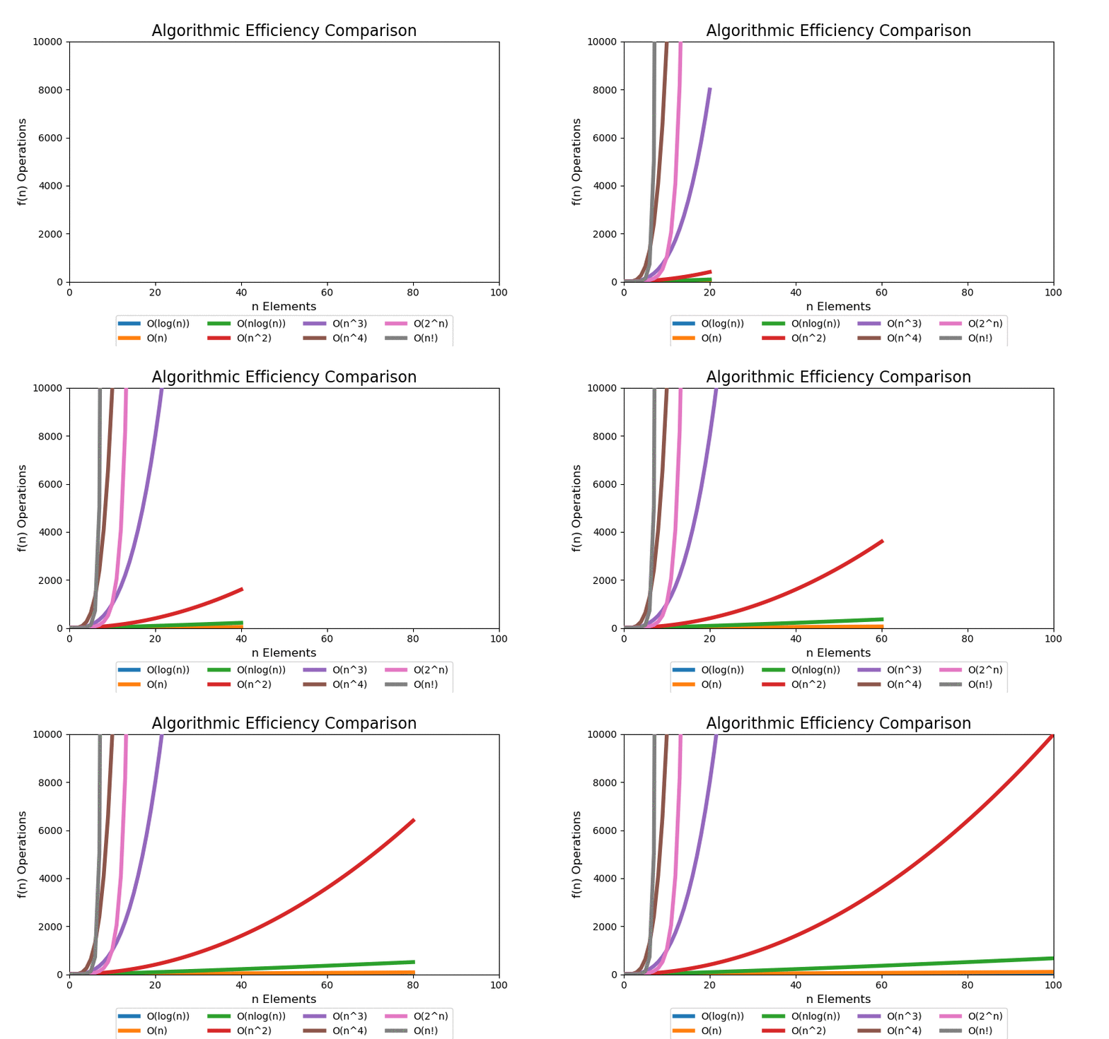
For a small data set, we can see quick divergence between the difference classes on a linear scale plot, but it is difficult to grasp the overall scale of growth and how different each class is. 100 elements is such a small data set that algorithms up to low polynomial time can be solved in an acceptable real time. However, when the data set grows into a large data set, even polynomial time algorithms become intractable.

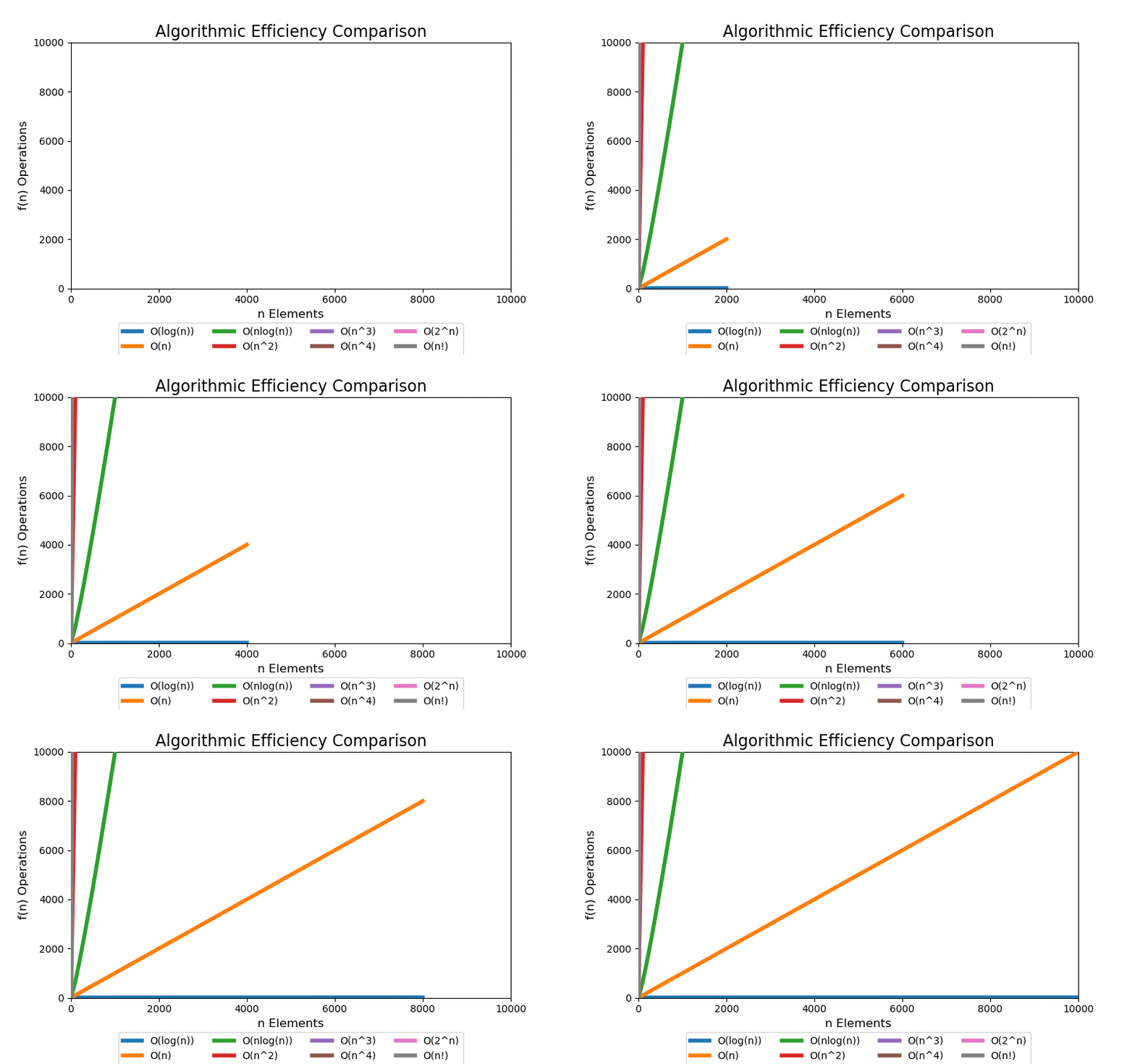
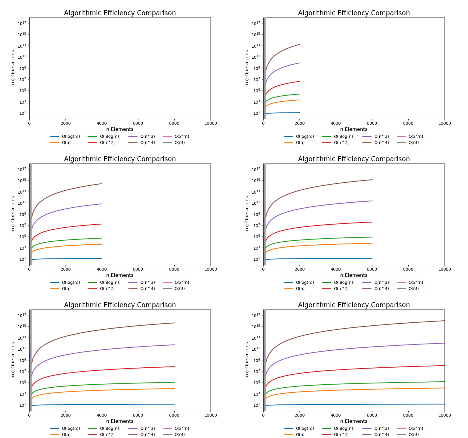
We are most concerned with large data sets. The following visualizations illustrate data sets up to a size of 10,000 elements. 10,000 elements can only marginally be considered a "large data" set as most modern applications are dealing with data containing with many orders of magnitude larger, i.e. billions and trillions of records. Regardless, at 10,000 records the pattern of extreme performance differences start to emerge in the visualizations.

With a linear scale plot, everything worse than loglinear is tightly grouped close to the y-axis and it is difficult to see differences.

If we scale the y-axis logrithmically, the asymptotic behavior starts to be more apparant. Both exponential and factorial are still off the chart at small values of n, but we can see that all other classes that have better asymptotic performance clearly start to flatten (on this scale) which help differentiate their differences in performance.