LOSSY COMPRESSION AND SCALAR QUANTIZATION
Abdou Youssef
-
Motivation
-
General Scheme of Lossy Compression
-
Illustration of the Effects of Transforms
and the Need for Quantization
-
Scalar Quantization
-
Types of Scalar Quantizers
-
Illustration of Quantizers
-
Optimal Non-Uniform Quantizers
(Max-Lloyd Quantizers)
-
Optimal Semi-Uniform Quantizers
Back to Top
1. Motivation
- Need for low bitrate
- Less than 0.2 bit per pixel for video
- Inadequacy of lossless compression
- Achievable compression ratio hardly above 2
- Achievable bitrate hardly below 4 bits per pixel
- Presence of visual redundancy that can be greatly exploited
Back to Top
2. General Scheme of Lossy Compression
- Approach
- Transform: Convert the data to the frequency domain
- Quantize: Under-represent the high frequencies
- Losslessly compress the quantized data
- Properties of transforms
- Decorrelation of data
- Separation of data into
- vision-sensitive data (low-frequency data)
- vision-insensitive data (high-frequency data)
- Various transforms achieve both properties
- Fourier Transform
- Discrete Cosine Transform (DCT)
- Other Fourier-like transforms: Haar, Walsh, Hadamard
- Wavelet transforms
- Properties of quantization
- Progressive under-representation of higher-frequency data
- Conversion of visual redundancy to symbol-level redundancy
that leads to high compression ratios
- Minimum and controlled distortion:
more errors in less sensitive regions
- Examples of quantizers
- Uniform scalar quantization
- Non-uniform scalar quantization
- Vector quantization (VQ)
Back to Top
3. Illustration of the Effects of Transforms
and the Need for Quantization
- The Lena Image
- The DCT transform of Lena
- An 8x8 block from inside the Lena image
| 247 | 108 | 247 | 119 | 119 | 119 | 118 | 108
|
| 72 | 118 | 118 | 108 | 118 | 108 | 119 | 119
|
| 209 | 4 | 108 | 108 | 118 | 108 | 119 | 118
|
| 108 | 247 | 108 | 118 | 119 | 118 | 108 | 119
|
| 119 | 247 | 247 | 119 | 108 | 118 | 119 | 119
|
| 108 | 247 | 247 | 119 | 247 | 108 | 118 | 119
|
| 118 | 119 | 247 | 118 | 108 | 118 | 119 | 119
|
| 108 | 108 | 247 | 108 | 119 | 108 | 119 | 108
|
- The Block's DCT:
| 13.9337 | 4.0995 | 8.3457 | 6.0095 | 0.8569 | 2.8970 | 1.2163 | 0.3561
|
| 2.5555 | 8.2141 | 8.1799 | 5.2586 | 5.5371 | 3.5972 | 2.6749 | 1.3947
|
| 8.3381 | 1.5359 | 2.1086 | 6.1568 | 4.4744 | 4.0792 | 3.3524 | 1.7280
|
| 2.4938 | 11.9743 | 6.7519 | 3.4772 | 5.5491 | 2.6686 | 1.5812 | 1.2808
|
| 0.3908 | 10.9625 | 14.6793 | 3.9725 | 1.2765 | 2.3745 | 1.5301 | 0.8110
|
| 3.2443 | 4.9893 | 13.1939 | 3.6871 | 7.6206 | 0.6060 | -0.3524 | 0.5137
|
| 2.6553 | -1.9329 | 4.6038 | 4.0076 | -1.4233 | 2.3443 | 1.5096 | 0.5551
|
| 1.4682 | -1.8891 | 2.4547 | 1.6346 | -0.7201 | 0.8214 | 0.7366 | -0.1023
|
- A 3D plot of the the Block's DCT is:
Back to Top
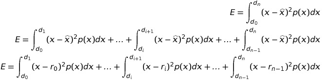
4. Scalar Quantization
- Definition of Quantization/Dequantization:
- A k-level quantizer is typically characterized by
k+1 decision levels
d0,d1, ... , dk, and by k
reconstruction levels
r0,r1, ... rk-1.
- The dis divide the range of data under
quantization into k consecutive intervals
[d0,d1) [d1,d2) ... [dk-1, dk).
- Each ri is in [di,di+1), and can be viewed as
the ``centroid'' of its interval.
- Quantizing a number x means locating the interval [di,di+1)
that contains x, and replacing x by index i. We simply write it as: Q(x)=i.
- Dequantization (in reconstruction)
is the process of replacing each index i by the value
ri. This approximates every original
number that was in interval [di,di+1) by
the centroid ri. We simply write it as DQ(i)=ri, or Q-1(i)=ri.
- A few quantizers assume that d0=-
 and dk=.
But in the majority of quantizers d0 and dk are finite numbers
representing the minimum and maximum value of the data being quantized.
and dk=.
But in the majority of quantizers d0 and dk are finite numbers
representing the minimum and maximum value of the data being quantized.
Back to Top
5. Types of Scalar Quantizers
- Uniform Quantizers
- All the decision intervals are of equal size
 =
(dk-d0)/k
=
(dk-d0)/k
- di=d0+i
- The reconstruction levels ri are the centers of the intervals
- Non-Uniform Quantizers: One or both of the following hold
- the decision intervals are not of equal size
- the reconstruction levels are not the centers of their intervals
- Semi-Uniform Quantizers
- Equal intervals
- The reconstruction levels are not necessarily the interval centers
Back to Top
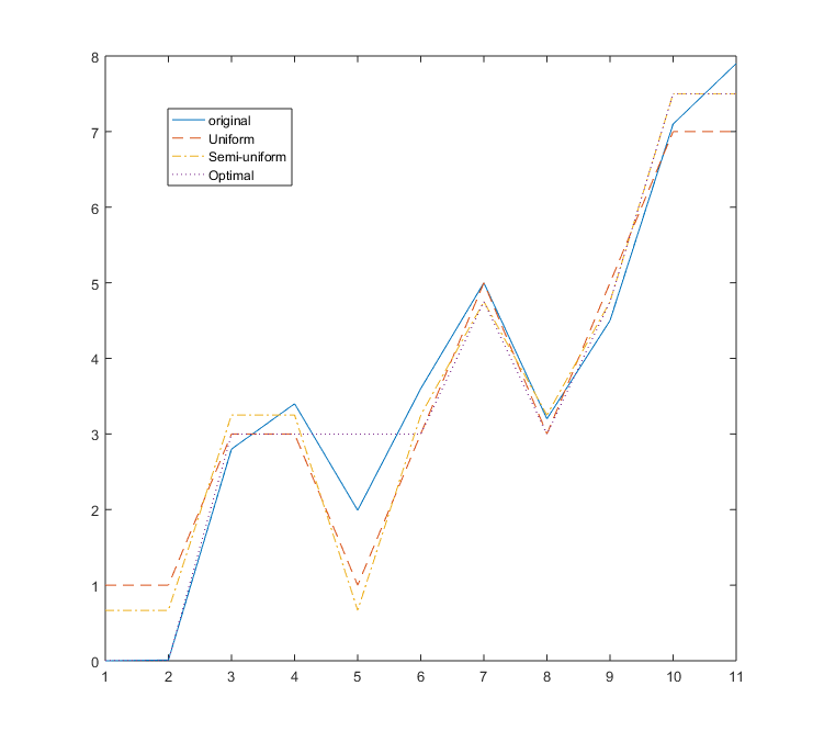
6. Illustration of Quantizers
- The 3 quantizers will be illustrated on a 1D example
- Signal X=[0 0.01 2.8 3.4 1.99 3.6 5 3.2 4.5 7.1 7.9]
- Denote by X' the quantized signal
- Unform Quantizer: The range 0-8 is divided into 4 equal intervals
| Original Signal X
| 0 | 0.01 | 2.8 | 3.4 | 1.99 | 3.6 | 5
| 3.2 | 4.5 | 7.1 | 7.9
|
| Quantized Signal X'
| 1 | 1 | 3 | 3 | 1 | 3 | 5 | 3 | 5 | 7 | 7
|
MSE=0.42
- Semi-Uniform Quantizer
| r0 | r1 | r2 | r3
|
| 2/3 | 3.25 | 4.75 | 7.5
|
| Original Signal X
| 0 | 0.01 | 2.8 | 3.4 | 1.99 | 3.6 | 5
| 3.2 | 4.5 | 7.1 | 7.9
|
| Quantized Signal X'
| 2/3 | 2/3 | 3.25 | 3.25 | 2/3 | 3.25 | 4.75 | 3.25 | 4.75 | 7.5 | 7.5
|
MSE=0.31
- Optimal Quantizer (to be derived later)
| d0 | d1 | d2 | d3 |
d4
|
| 0 | 1.5 | 3.87 | 6.125 | 8
|
| r0 | r1 | r2 | r3
|
| 0.005 | 2.998 | 4.75 | 7.5
|
| Original Signal X
| 0 | 0.01 | 2.8 | 3.4 | 1.99 | 3.6 | 5
| 3.2 | 4.5 | 7.1 | 7.9
|
| Quantized Signal X'
| 0.005 | 0.005 | 2.998 | 2.998 | 2.998 | 2.998
| 4.75 | 2.998 | 4.75 | 7.5 | 7.5
|
MSE=0.18
- Graphic comparison of the sigal and its quantizations
 Back to Top
7. Optimal Non-Uniform Quantizers
(Max-Lloyd Quantizers)