13.1
What problem does the Harrow–Hassidim–Lloyd (HHL) Algorithm solve?
The HHL algorithm seeks to approximate a solution to simultaneous
linear equations:
the well-known
\({\bf Ax} = {\bf b}\) problem:
- Classically, we describe "solving simultaneous linear equations" as
solving for \({\bf x}\) in
$$
{\bf Ax} \eql {\bf b}
$$
Here:
- \({\bf A}\) is an \(N \times N\) matrix
$$
{\bf A} \eql \mat{
A_{11} & A_{12} & \cdots & A_{1N} \\
A_{21} & A_{22} & \cdots & A_{2N} \\
\vdots & \vdots & \vdots & \vdots \\
A_{N1} & A_{N2} & \cdots & A_{NN} \\
}
$$
- \({\bf b}\) is an \(N \times 1\) vector
$$
{\bf b} \eql \mat{b_1 \\ b_2\\ \vdots\\ b_N}
$$
- \({\bf x}\) is an \(N \times 1\) vector of "variables"
$$
{\bf x} \eql \mat{x_1 \\ x_2\\ \vdots\\ x_N}
$$
whose equation-satisfying values we seek.
- In linear-equation form this is:
$$\eqb{
A_{11} x_1 + \ldots + A_{1N}x_N & \eql & b_1 \\
A_{21} x_1 + \ldots + A_{2N}x_N & \eql & b_2 \\
& \vdots & \\
A_{N1} x_1 + \ldots + A_{NN}x_N & \eql & b_N \\
}$$
Which we can write in the familiar matrix-vector form:
$$
\mat{
A_{11} & A_{12} & \cdots & A_{1N} \\
A_{21} & A_{22} & \cdots & A_{2N} \\
\vdots & \vdots & \vdots & \vdots \\
A_{N1} & A_{N2} & \cdots & A_{NN} \\
}
\mat{x_1 \\ x_2\\ \vdots\\ x_N}
\eql
\mat{b_1 \\ b_2\\ \vdots\\ b_N}
$$
Or compactly as
$$
{\bf Ax} \eql {\bf b}
$$
- For example (\(N=3\)):
- Suppose we have the equations
$$\eqb{
2x_1 & - & 3x_2 & + & 2x_3 & \eql & 5\\
-2x_1 & + & x_2 & & & \eql & -1\\
x_1 & + & x_2 & - & x_3 & \eql & 0
}$$
- In matrix form, this becomes
$$
\mat{2 & -3 & 2\\
-2 & 1 & 0\\
1 & 1 & -1}
\vecthree{x_1}{x_2}{x_3}
\eql
\vecthree{5}{-1}{0}
$$
- What we would like to do, of course, is solve for \({\bf x}\):
$$
{\bf x} \eql {\bf A}^{-1} {\bf b}
$$
- What HHL algorithms seeks to do is approximate a solution
$$
{\bf x} \; \approx \; {\bf A}^{-1} {\bf b}
$$
Let's review the classical context for this problem:
- Writing
$$
{\bf x} \eql {\bf A}^{-1} {\bf b}
$$
suggests that we first find the matrix inverse \({\bf A}^{-1}\)
and simply multiply into \({\bf b}\).
- Alternatively, we also learned how to iterate through
Gaussian elimination to solve for \({\bf x}\) directly.
- A host of classical algorithms has evolved to solve
\({\bf Ax}={\bf b}\) exactly in general and for various special cases:
- (General) Gaussian elimination via LU-Decomposition
- (General) QR factorization
- (Symmetric \({\bf A}\)) Cholesky decomposition
- Iterative methods solve approximately, with accuracy increasing
with iteration:
- Gauss-Seidel method
- Conjugate gradient method
- Jacobi method
- Finally, when \({\bf Ax}={\bf b}\) has no exact solution (example: non-square matrices), a nearest solution can be found:
- Least-squares algorithm
- SVD algorithm
- How long do these algorithms take?
- In general, the algorithms take \(O(N^3)\).
- In special cases, where \({\bf A}\) has special structure,
some algorithms can run in \(O(N^2)\).
- Just as many algorithms exist to find the inverse \({\bf A}^{-1}\).
- An advantage with first solving for \({\bf A}^{-1}\):
- Once we've solved for \({\bf A}^{-1}\), this can be applied
to different \({\bf b}\)'s.
- This is common in many applications.
- What HHL tries to do: directly solve for \({\bf x}\) approximately in time \(O(\log N)\)
\(\rhd\)
Potentially, an exponential speed up
The HHL algorithm is somewhat complicated, with many details and assumptions. We'll do this in steps.
13.2
HHL: A high-level overview
Recall the goal:
- Conventional notation:
Given real matrix \({\bf A}\) and real vector \({\bf b}\),
solve for \({\bf x}\) where \({\bf Ax}={\bf b}\).
- In Dirac notation:
Given real matrix \(A\) and real vector \(\kt{b}\),
solve for \(\kt{x}\) where \(A\kt{x} = \kt{b}\).
- Clearly, \(\kt{x} = A^{-1} \kt{b}\)
- Here, we are describing a classical problem using Dirac notation.
- With the various algorithms we've seen, one would imagine the
quantum version would look like this:
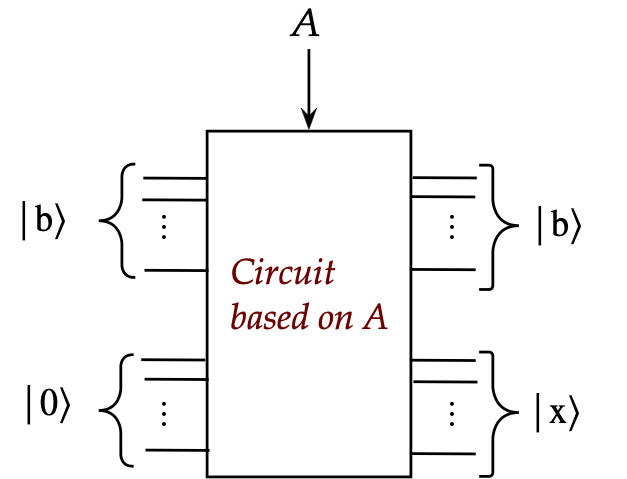
- However, it will turn out to be:
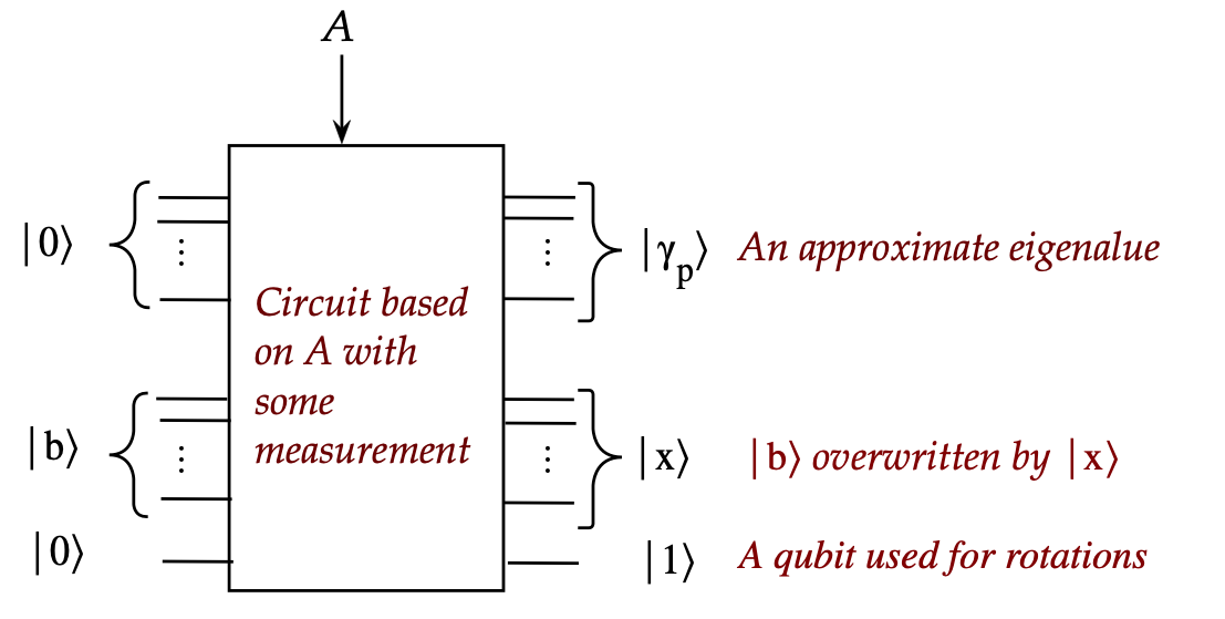
The HHL algorithm is based on two key ideas:
- An analysis that expresses the solution \(\kt{x}\)
in terms of the eigenvectors and eigenvalues of \(A\):
- Suppose \(A\) has eigenvectors are \(\kt{u_1}, \kt{u_2}, \ldots, \kt{u_N}\) with corresponding eigenvalues \(\lambda_1,\lambda_2,\ldots, \lambda_N\)
- Express \(\kt{b}\) in terms of the eigenvectors:
$$
\kt{b} \eql \sum_j \beta_j \kt{u_j}
$$
(\(\beta_j\) are the coefficients)
- It will turn out (see below) that
$$
\kt{x} \eql
\sum_j \lambda_j^{-1} \beta_j \kt{u_j}
$$
- Quantum operations that arrange for the inverse eigenvalues
\(\lambda_j^{-1}\) to appear next to the corresponding \(\beta_j\)'s:
- The vector \(\kt{b}\) is loaded into a multi-qubit register
- Operations are performed so that the register will eventually
approximately contain \(\sum_j \lambda_j^{-1} \beta_j \kt{u_j}\)
(That is, approximately \(\kt{x}\))
Note:
- Note: HHL does not explicitly calculate the \(\kt{u_j}\)'s.
- They are used only in the theory behind the algorithm
Let's flesh out a few details:
- Suppose \(A\) is Hermitian (symmetric, since it's real).
(We'll visit this assumption later.)
- Then by the spectral theorem (Module 2),
\(A\) has
- eigenvectors \(\kt{u_1}, \kt{u_2}, \ldots, \kt{u_N}\)
- with corresponding real eigenvalues \(\lambda_1,\lambda_2,\ldots, \lambda_N\)
- We know (Module 2) that \(A\) can be written in terms
of eigenvector projectors:
$$
A \eql \sum_j \lambda_j \otr{u_j}{u_j}
$$
- Then (see exercise below),
$$
A^{-1} \eql \sum_j \lambda_j^{-1} \otr{u_j}{u_j}
$$
- Next, since \(\kt{u_1}, \kt{u_2}, \ldots, \kt{u_N}\)
form a basis, any vector \(\kt{b}\) can be written as a linear combination
$$
\kt{b} \eql \sum_j \beta_j \kt{u_j}
$$
- Applying \(A^{-1} \kt{b}\)
$$\eqb{
\kt{x} & \eql & A^{-1} \kt{b} \\
& \eql &
\parenl{ \sum_j \lambda_j^{-1} \otr{u_j}{u_j} }
\parenl{ \sum_k \beta_k \kt{u_k} } \\
& \eql &
\sum_j \lambda_j^{-1} \beta_j \kt{u_j}
}$$
- At the moment, this is only analysis.
In-Class Exercise 1:
Show that \({\bf A}^{-1} = \sum_j \lambda_j^{-1} \otr{u_j}{u_j}\)
by multiplying \({\bf A}^{-1} {\bf A}\).
Let's now consider what a quantum circuit must do:
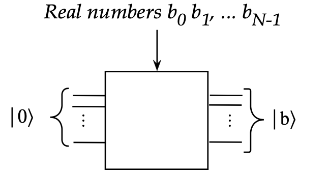
- First, we'll want a way to load the vector \(\kt{b}\)
into a multi-qubit register:
- We are given \(N\) real numbers \(\kt{b} = (b_1,\ldots,b_{N})\)
- Which we will sometimes relabel as \(\kt{b} = (b_0,\ldots,b_{N-1})\)
(to align with standard-basis numbering)
- We can now write
$$
\kt{b} \eql \mat{b_0 \\ b_1 \\ \vdots\\ b_{N-1}}
\eql \sum_j b_j \kt{j}
$$
- How many qubits?
Since there are \(N\) basis vectors \(\kt{u_1}, \kt{u_2}, \ldots, \kt{u_N}\), we'll need \(n = \lceil\log N\rceil\) qubits so that
$$\eqb{
\kt{b} & \eql & \sum_{j=0}^{N-1} b_j \kt{j} \\
& \eql & b_0\kt{0} + b_1\kt{1} + \ldots + b_{N-1}\kt{N-1}\\
& \eql & b_0\kt{0} + b_1\kt{1} + \ldots + b_{2^n-1}\kt{2^n-1}\\
}$$
(We'll assume \(N=2^n\) exactly, for simplicity.)
- In indexing, we'll leave out limits \(j \in \{1 \ldots N\}\) or
\(j \in \{0 \ldots N-1\}\) where the context makes it clear.
- Note: we are assuming \(\magsq{b} = 1\) since we want \(\kt{b}\)
to be a multi-qubit state:
- There is no guarantee that the input data \((b_0,\ldots,b_{N-1})\)
is such that \(b_0^2 + \ldots + b_{N-1}^2 = 1\).
(We'll address this assumption later.)
- We will need a way to load a quantum register with \(\kt{b}\)
\(\rhd\)
Module 14 will show how
- Assuming we can load \(\kt{b}\), we'll have a register with
$$
\kt{b} \eql \sum_{j} b_j \kt{j} \eql \sum_j \beta_j \kt{u_j}
$$
Note:
- The register is loaded with \(\kt{b}\) using the given
components \((b_0,\ldots,b_{N-1})\)
- We do not know (nor will need to know)
the eigenvectors \(\kt{u_1}, \kt{u_2}, \ldots, \kt{u_N}\)
- Nor do will we need to know the \(\beta_j\)'s
- The right side merely shows that we can mathematically
express \(\kt{b}\) in terms of the \(\kt{u_j}\)'s
- We will create quantum operations that produce the reciprocal eigenvalues
$$
\sum_j \lambda_j^{-1} \beta_j \kt{u_j} \eql \kt{x}
$$
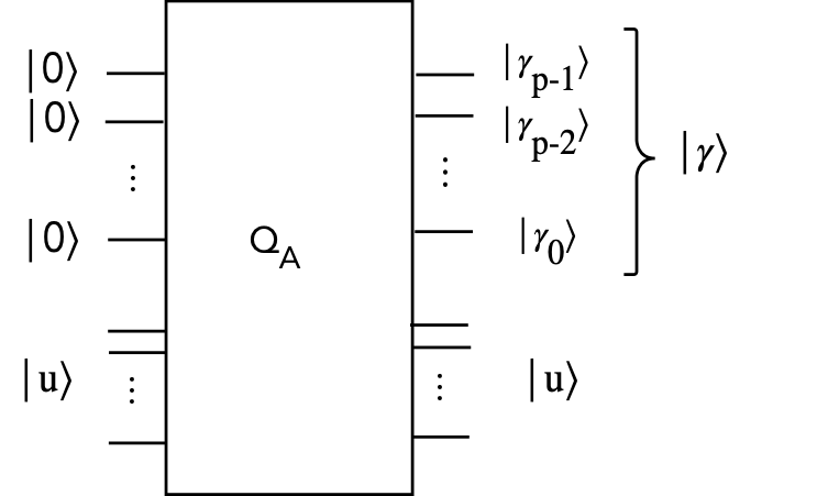
- Suppose we have a quantum operator \(Q_A\) (that depends on \(A\))
such that
$$
Q_A \kt{00\ldots 0} \kt{u_j} \eql \kt{\gamma_{j,p}} \kt{u_j}
$$
Here
- \(u_j\) is an eigenvector of \(A\)
- The qubits \(\kt{00\ldots 0}\) are \(p\) ancillae qubits (a register)
- After the operator is applied, a \(p\)-digit approximation of
scaled eigenvalue \(\gamma_j\) called \(\kt{\gamma_{j,p}}\)
appears in the ancilla register
- Then, if we apply this operator to \(\kt{b}\), we'd have
$$\eqb{
Q_A \kt{b} & \eql & Q_A \, \kt{00\ldots 0} \, \parenl{ \sum_j \beta_j \kt{u_j} } \\
& \eql &
\sum_j \beta_j Q_A \kt{00\ldots 0} \kt{u_j} \\
& \eql &
\sum_j \beta_j \kt{\gamma_{j,p}} \kt{u_j} \\
}$$
- Finally, we need to use the eigenvalue in the register
to result in multiplying each coefficient by its reciprocal:
$$\eqb{
\sum_j \beta_j \kt{\gamma_{j,p}} \kt{u_j}
& \;\; \rightarrow \;\; &
\sum_j \beta_j \lambda_j^{-1} \kt{00\ldots 0} \kt{u_j} \\
& \eql &
\kt{00\ldots 0} \sum_j \beta_j \lambda_j^{-1} \kt{u_j} \\
& \eql &
\kt{00\ldots 0} \kt{x}
}$$
where we now have the (approximate) solution \(\kt{x}\) in the second register.
- The tricky parts are:
- How does one build an operator like \(Q_A\)?
- How does one build a circuit to use a qubit-register state
to produce a corresponding coefficient (a number)?
Before getting into the weeds, let's examine the assumptions
13.3
HHL assumptions
Assumption 1: \(A\) is symmetric
- Clearly, this is not a reasonable assumption when given a generic
\({\bf Ax}={\bf b}\) problem.
- However, if \(A\) is not symmetric, then
$$
\bar{A} \eql \mat{ 0 & A^T\\ A & 0}
$$
is symmetric.
- For example, if
$$
A \eql \mat{a & b\\ c & d}
$$
(which is not symmetric) then
$$
\bar{A} \eql \mat{0 & 0 & a & c\\
0 & 0 & b & d\\
a & b & 0 & 0\\
c & d & 0 & 0\\}
$$
is symmetric.
- If we instead solve \({\bf \bar{A}\bar{x}}={\bf \bar{b}}\),
we can reconstruct
the solution to \({\bf Ax}={\bf b}\), as the exercise below shows.
- Thus, one can solve a larger system with a symmetric \(\bar{A}\).
- Why do we need \(A\) to be symmetric?
- First, we need \(A\) to have real eigenvalues with
eigenvectors that form a basis.
\(\rhd\)
The whole algorithm is premised on this assumption
- Next, as we'll see shortly, if \(A\) is Hermitian then
$$
U \eql e^{iA}
$$
is unitary.
- Moreover, \(U\) has the same eigenvectors as \(A\) but with
different eigenvalues:
$$
U\kt{u_j} \eql e^{i\lambda_j} \kt{u_j}
$$
- Thus, if we build a circuit for applying \(U\), we can
make \(e^{i\lambda_j}\) appear as a coefficient.
Note: we eventually need \(\lambda_j^{-1}\)'s as coefficients
In-Class Exercise 2:
Using \(A=\mat{a & b\\ c & d}\) example, show how to set up
\({\bf \bar{A}\bar{x}}={\bf \bar{b}}\), with \({\bf \bar{b}}\)
constructed from \({\bf b}\), so that \({\bf x}\)
can be inferred from \({\bf \bar{x}}\)
Assumption 2: \(\kt{b}\) has unit magnitude
- Here, we're making the assumption that with
$$
\sum_j \magsq{b_j} \eql 1
$$
- Define
$$
\kt{\bar{b}} \eql \frac{1}{\mag{b}} \kt{b}
$$
so that \(\kt{\bar{b}}\) has unit magnitude
- Suppose we now solve
$$
A \kt{\bar{x}} \eql \kt{\bar{b}}
$$
- Then, one can recover \(\kt{x}\) from \(\kt{\bar{x}}\)
(Exercise below)
In-Class Exercise 3:
Show that this is the case.
Assumption 3: \(\kt{x}\) has unit magnitude
- Clearly, qubits have unit-magnitude vectors.
\(\rhd\)
The output will have unit-magnitude
- But the true solution \(\kt{x}\) may not in fact have
unit magnitude.
- Suppose the quantum circuit produces
$$
\kt{y} \eql \frac{1}{\mag{x}} \kt{x}
$$
and suppose that \(\kt{y}\) is extracted from the quantum circuit.
- Then, the classical multiplication
$$\eqb{
A \kt{y} & \eql & A \frac{1}{\mag{x}} \kt{x} \\
& \eql &
\frac{1}{\mag{x}} \: A\kt{x} \\
& \eql &
\frac{1}{\mag{x}} \: \kt{b}
}$$
From which (since \(\mag{y} = 1\))
$$
\mag{x} \eql \mag{b}
$$
And from which
$$
\kt{x} \eql \mag{x} \kt{y}
$$
- Thus, at the moment, this appears to not be a limiting assumption.
- But ... see Assumption 6 below
Assumption 4: \(\kt{b}\) can be loaded efficiently
- Thus, far we have not studied how to load arbitrary (unit-magnitude)
vectors into a qubit register:
- Since this is a generally useful operation across algorithms,
we'll devote Module-14 to this problem.
- However, notice that it will take at least as much time
as there are coefficients \(\kt{b} = (b_0,\ldots,b_{N-1})\).
Assumption 5: \(U=e^{iA}\) can be implemented efficiently
- Given the matrix \(A\) we are ultimately, going to build a unitary
\(U_A = e^{iA}\) so that
$$
U_A \kt{u_j} \eql e^{i\lambda_j} \kt{u_j}
$$
- Apply the unitary \(U_A\) extracts the eigenvalues
- These appear in exponentiated form
- We will see later
how the eigenvalues can then be further "un-exponentiated"
- The assumption here is that an efficent unitary circuit
can be constructed from \(U=e^{iA}\), where \(A\) is itself large.
- It is not clear this can always be done.
- This is a specialized subtopic called Hamiltonian simulation,
which can be efficient provided \(A\) has few nonzero elements.
Assumption 6: measurement
- Suppose HHL produces \(\kt{x}\) in a register.
- That is, the register contains
$$
\kt{x} \eql \sum_j x_j \kt{j}
$$
- How exactly do we extract the real numbers \(x_0,\ldots x_{N-1}\)?
- Measuring repeatedly to estimate \(x_j\)'s will need
many, many repetitions.
Assumption 7: efficiency
- Remember the exponential speedup claim?
\(\rhd\)
Solving for \(\kt{x}\) takes time \(\log N\)
- But this cannot be if:
- Loading \(\kt{b}\) takes at least \(N\) time
- Constructing symmetric \(A\) takes at least \(O(N^2)\) time
- Extracting \(x_j\)'s from \(\kt{x}\) takes many measurements
- It is instead best to understand efficiency differently where
HHL is part of a larger quantum computation where
- \(\kt{b}\) is already in a register
- The goal is to produce \(\kt{x}\) instead of its
standard-basis coordinates \(x_0,\ldots,x_{N-1}\)
- This \(\kt{x}\) is presumably useful in later parts of the
larger computation
Summary of assumptions:
- We will henceforth make all the assumptions above.
- The real goal of studing HHL:
- It uses new building blocks that could be useful in future algorithms
- It demonstrates how to work with eigenvalues in a quantum circuit
13.4
An important building block: the QPE algorithm
Let's review the QPE algorithm (Module 12) as a building block:
- Consider the \(j\)-th eigenpair:
- \(\kt{u} \in \{u_0,\ldots,u_{N-1}\}\) = an eigenvector of \(A\)
- \(\kt{\lambda}\) = corresponding eigenvalue
- Let
$$
\gamma_\lambda \eql 0.\gamma_{p-1}\gamma_{p-2}\ldots\gamma_0
$$
be a \(p\) digit number such that
$$
2\pi(0.\gamma_{p-1}\gamma_{p-2}\ldots\gamma_0) \;\;\approx\;\; \lambda
$$
Here:
- Think of this as starting with \(\lambda\), then calculating
$$
\gamma^\prime \eql \frac{\lambda}{2\pi}
$$
- We'll assume, as we did in Module 12, that \(0 \lt \gamma^\prime \lt 1\)
- Then, \(\gamma^\prime\) can be written approximately
in binary form, truncating after \(p\) digits:
$$
\gamma^\prime \;\;\approx\;\;
0.\gamma_{p-1}\gamma_{p-2}\ldots\gamma_0
$$
This is what we're calling \(\gamma_\lambda\)
- Clearly, \(\gamma_\lambda\) depends on \(\lambda\)
- Note:
- The choice of \(p\) is hardware dependent.
- High \(p\) is better, but will take more time (gates)
- We will use the notation
$$
\kt{\gamma} \eql \kt{\gamma_{p-1}\gamma_{p-2}\ldots\gamma_0}
\eql \kt{\gamma_{p-1}} \kt{\gamma_{p-2}} \ldots \kt{\gamma_0}
$$
to indicate the standard-basis vector formed from the digits.
- Whereas \(\gamma\) is a real number, we're only using
\(\kt{\gamma}\) as a shorthand for the binary digits.
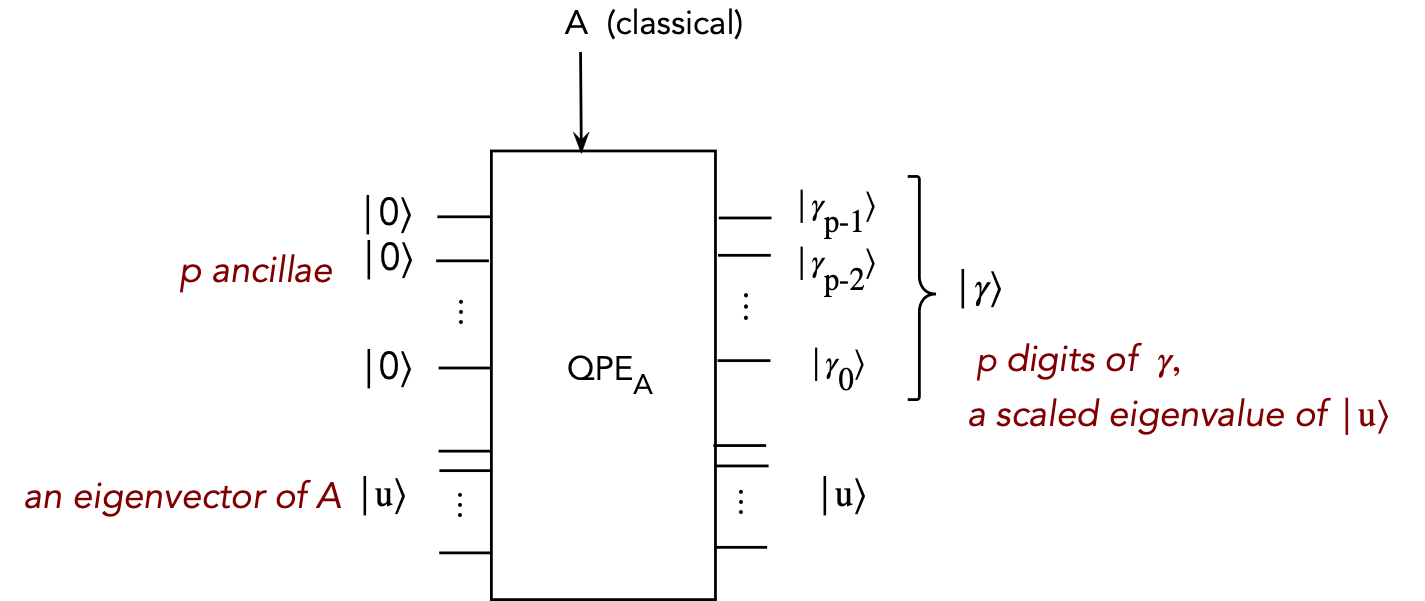
- The QPE circuit produces this vector as output in the top qubits,
as seen.
- For HHL, we're going to need more, but this is a first step.
- Next, let's write this circuit compactly as:
$$
Q_A \kt{0}^{\otimes p} \kt{u} \eql
\kt{\gamma_{p-1}} \kt{\gamma_{p-2}} \ldots \kt{\gamma_{0}}
\: \kt{u}
$$
Or
$$
Q_A \kt{0}^{\otimes p} \kt{u} \eql
\kt{\gamma} \: \kt{u}
$$
- At the risk of a bit of confusion, we'll use two
different subscripts for \(\gamma\):
- For "which bit"
$$
\gamma_p \eql p\mbox{-th bit of }\gamma
$$
- And for which eigenvector:
$$
\gamma_j \eql \gamma \mbox{ corresponding to eigenvector } u_j
$$
- When we need to specify the \(p\)-th bit of the the \(j\)-th
\(\gamma\), we'll use
$$
\gamma_{j,p} \eql p\mbox{-th bit of \(j\)-th } \gamma
$$
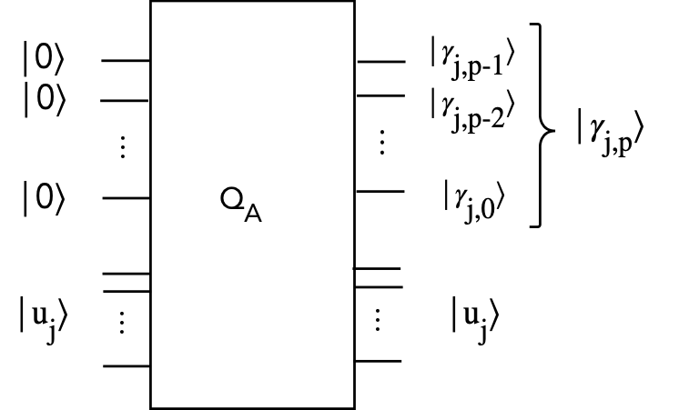
Thus,
$$
\kt{\gamma_j} \eql \kt{\gamma_{j,p-1}\gamma_{j,p-2}\ldots\gamma_{j,0}}
\eql \kt{\gamma_{j,p-1}} \kt{\gamma_{j,p-2}} \ldots \kt{\gamma_{j,0}}
$$
And so, the circuit diagram looks like:
- From this, we can see what happens if we feed a linear
combination of \(\kt{u_j}\)'s:
$$\eqb{
Q_A \kt{0}^{\otimes p} \: \sum_j \beta_j \kt{u_j}
& \eql &
\sum_j Q_A \kt{0}^{\otimes p} \: \beta_j \kt{u_j} \\
& \eql &
\sum_j \beta_j Q_A \kt{0}^{\otimes p} \: \kt{u_j} \\
& \eql &
\sum_j \beta_j \kt{\gamma_j} \: \kt{u_j}
}$$
where the \(\gamma\)'s are now indexed by \(j\) since there is one
for each eigenvector.
- Compare this to our desired solution:
$$\eqb{
\kt{x} & \eql & A^{-1} \kt{b} \\
& \eql &
\parenl{ \sum_j \lambda_j^{-1} \otr{u_j}{u_j} }
\parenl{ \sum_k \beta_k \kt{u_k} } \\
& \eql &
\sum_j \lambda_j^{-1} \beta_j \kt{u_j}
}$$
Thus, we somehow need to use \(\kt{\gamma(j)}\) to
create the constant \(\lambda_j^{-1}\)
We're going to explore two approaches and along the way, develop
some building blocks useful in other quantum algorithms.
13.5
A building block: multi-controlled rotations
Let's begin with a simple rotation gate and obtain
a multi-controlled version:
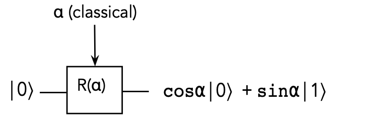
- Define
$$
R(\alpha) \eql
\mat{ \cos\alpha & -\sin\alpha\\
\sin\alpha & \cos\alpha}
$$
(This is the gate \(R_Y(2\alpha)\) from Module 6.)
- Then,
$$
R(\alpha) \kt{0} \eql \cos\alpha \kt{0} + \sin\alpha \kt{1}
$$
Pictorially:
- A singly-controlled version:
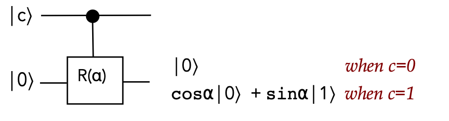
Which we can write as
$$
R^c(\alpha) \kt{c}\kt{0} \eql \left\{
\begin{array}{l}
\kt{0}\kt{0} & \;\;\; & c=0\\
\kt{1}\: \left(\cos\alpha \kt{0} + \sin\alpha\kt{1} \right)& \;\;\; & c=1\\
\end{array}
\right.
$$
- A multiply-controlled example:
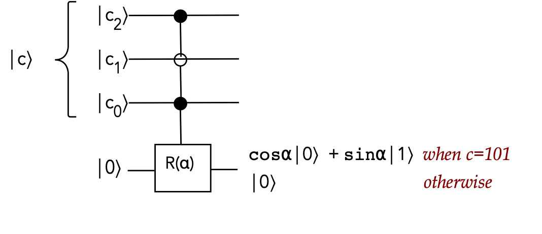
In this example:
- There are 3 control qubits
- Two are \(\kt{1}\)-activated, one is \(\kt{0}\)-activated
- We will be interested in the general case with \(p\)
control qubits, as in this example:
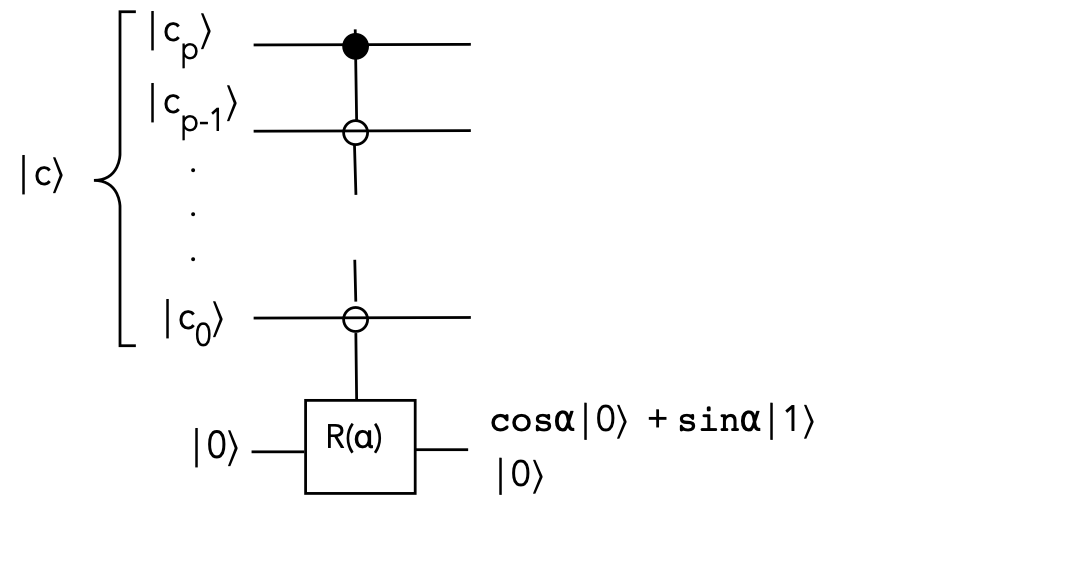
The rotation is activated when the control bits match the
circuit's controls (\(0\) or \(1\)).
- How many gates are required?
- From Module 7 (section 7.4): one can use \(p-1\) additional
qubits in \(p\) stages
- The final singly-controlled gate will itself need to
implemented using standard gates (Section 7.2)
- Alternatively, one can describe the \(2^{p+1} \times 2^{p+1}\)
unitary and try and optimize its decomposition into small gates.
13.6
Approach #1: HHL via multi-controlled rotations
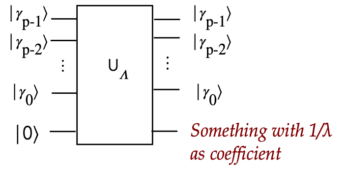
First, we'll set up a higher-level circuit goal:
Designing the circuit for \(U_\Lambda\):
- We'll use an example to illustrate with \(p=3\) and \(c=0.5\).
- There are \(2^p = 2^3 = 8\) possible binary digit
combinations for \(\gamma_2 \gamma_1 \gamma_0\):
$$
\begin{array}{|c|c|c|c|}\hline\hline
\gamma_2 \gamma_1 \gamma_0 & \lambda & \frac{c}{\lambda} &
\alpha = \sin^{-1}(\frac{c}{\lambda}) \\\hline
000 & & & \\
001 & 0.785 & 0.637 & 0.690 \\
010 & 1.570 & 0.318 & 0.324 \\
011 & 2.356 & 0.212 & 0.214 \\
100 & 3.142 & 0.159 & 0.160 \\
101 & 3.927 & 0.127 & 0.128 \\
110 & 4.712 & 0.106 & 0.106 \\
111 & 5.498 & 0.090 & 0.091 \\\hline
\end{array}
$$
- The 2nd column has each possible \(\lambda = 2\pi(0.\gamma_2 \gamma_1 \gamma_0)\)
- For example, \(3.927 = 2\pi(0.101_{\mbox{binary}}) = 2\pi(0.625_{\mbox{decimal}})\)
- With \(c=0.5\) arbitrarily chosen, we get the 3rd column.
- The 4th column is calculated for reasons described next.
- We eliminate \(000\) because it gives \(\lambda = 0\)
- For any \(\lambda\), suppose we calculate
$$
\alpha \eql \sin^{-1} \left( \frac{c}{\lambda} \right)
$$
and suppose we have a rotation gate that performs
$$
R(\alpha) \eql \cos\alpha\:\kt{0} \; + \; \sin\alpha\:\kt{1}
$$
Then
$$\eqb{
R(\alpha)\:\kt{0}
& \eql & \cos\alpha \: \kt{0} \; + \; \sin\alpha \: \kt{1} \\
& \eql &
\cos\alpha\:\kt{0} \; + \;
\sin \sin^{-1} \left( \frac{c}{\lambda} \right) \:\kt{1} \\
& \eql &
\cos\alpha\:\kt{0} \; + \; \frac{c}{\lambda} \: \kt{1} \\
& \eql &
c^\prime \kt{0} \; + \; \frac{c}{\lambda} \: \kt{1} \\
& \eql & \kt{\phi} \\
}$$
Where \(c^\prime\) was defined earlier and \(\kt{\phi}\) is just
the name we gave to this last vector.
(See the exercise below for why we get \(c^\prime\) in the last-but-one step.)
- Thus, each
\(\lambda = 2\pi(0.\gamma_2 \gamma_1 \gamma_0)\)
combination results in a different angle \(\alpha\) for a rotation gate.
- We need a way to let each \(\gamma_2 \gamma_1 \gamma_0\)
decide which \(\alpha\) to apply
\(\rhd\)
We know how to do this: using multi-controlled rotations!
- Let's use the names \(\alpha_{001}, \alpha_{010}, \ldots, \alpha_{111}\)
for the 7 angles in the table above (in radians).
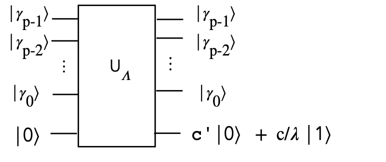
- We can now draw the circuit for \(U_\Lambda\):
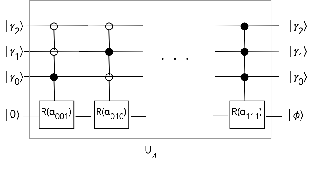
- Algebraically,
$$
U_\Lambda \kt{\gamma_2 \gamma_1 \gamma_0} \: \kt{0}
\eql
\kt{\gamma_2 \gamma_1 \gamma_0}
\: \left( c^\prime \kt{0} \; + \; \frac{c}{\lambda} \: \kt{1} \right)\\
$$
- Next, suppose we measure the last qubit:
- There are two possible (appropriately normalized) outcomes:
$$
\kt{\gamma_2 \gamma_1 \gamma_0} \: c^\prime \kt{0}
\;\;\;\;\; \mbox{or} \;\;\;\;\;
\kt{\gamma_2 \gamma_1 \gamma_0} \: \frac{c}{\lambda} \kt{1}
$$
- If we get \(\kt{0}\) as the last-qubit outcome, we'll discard
the entire outcome.
- If we keep the \(\kt{1}\) outcome, we get
$$
\frac{c}{\lambda} \: \kt{\gamma_2 \gamma_1 \gamma_0} \: \kt{1}
$$
Think of this as a way to get the desired coefficient \(\frac{c}{\lambda}\).
In-Class Exercise 5:
How did the coefficient of \(\kt{0}\) become \(c^\prime\) in the last-but-one
step of the derivation in applying \(R(\alpha)\) to \(\kt{0}\)?
We now have all the pieces for the HHL algorithm:
- First, let's start with the following circuit:
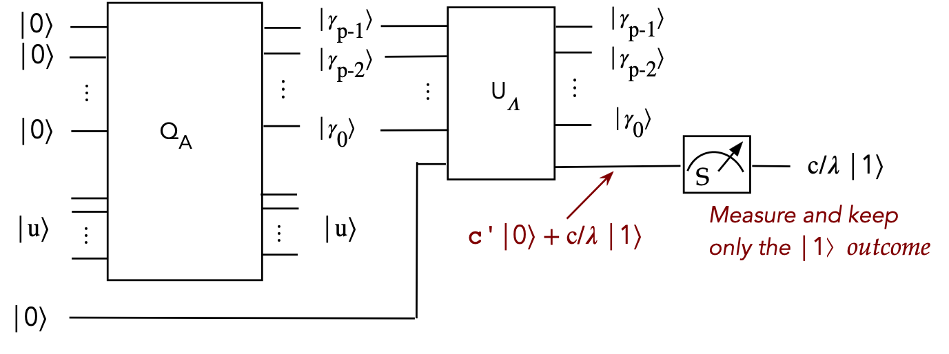
- The input consists of \(p\) ancillae and an eigenvector \(\kt{u}\)
of \(A\).
- The first \(Q_A\) produces a \(p\)-digit approximation of
the eigenvalue.
- These digits, together with a new ancilla are fed into \(U_\Lambda\)
- This produces an ancilla with different coefficients for
\(\kt{0}\) and \(\kt{1}\)
- We measure this ancilla, and keep the \(\kt{1}\) outcome
- Note:
- We've drawn \(U_\Lambda\) as we've done before.
- The \(\kt{u}\) output of \(Q_A\) does not go into \(U_\Lambda\)
- Technically, we could take \(\kt{u}\) as input to \(U_\Lambda\)
but not use it.
- Let's describe circuit's action algebraically:
$$\eqb{
U_\lambda \: Q_A \: \kt{0}^{\otimes p} \: \kt{u} \: \kt{0}
& \eql &
U_\lambda \: \kt{\gamma_{p-1}\ldots\gamma_0} \: \kt{u} \: \kt{0}
& \mbx{Applying \(Q_A\)} \\
& \eql &
\kt{\gamma_{p-1}\ldots\gamma_0} \: \kt{u} \:
\left(\frac{c}{\lambda} \: \kt{1} \right)
& \mbx{Measuring and keeping \(\kt{1}\)} \\
& \eql &
\frac{C}{\lambda} \kt{\gamma_{p-1}\ldots\gamma_0} \: \kt{u} \:
\kt{1}
& \mbx{Move constant out, normalize} \\
& \eql &
\frac{C}{\lambda} \kt{\gamma} \: \kt{u} \:
\kt{1}
& \mbx{Shorter form} \\
}$$
Note:
- Here, \(C\) represents a normalization constant that absorbs \(c\).
- To declutter, we've left out the identity operators in the tensored versions
of \(U_\Lambda\) and \(Q_A\).
- Next, let's use \(\kt{b}\) instead of \(\kt{u}\)
$$\eqb{
U_\lambda \: Q_A \: \kt{0}^{\otimes p} \: \kt{b} \: \kt{0}
& \eql &
U_\lambda \: Q_A \: \kt{0}^{\otimes p} \:
\left( \sum_j \beta_j \kt{u_j} \right) \: \kt{0}
& \mbx{Express \(\kt{b}\) in terms of the eigenvectors \(\kt{u_j}\)}\\
& \eql &
\sum_j \: U_\lambda \: Q_A \: \kt{0}^{\otimes p} \:
\beta_j \kt{u_j} \: \kt{0}
& \mbx{Operator movement}\\
& \eql &
\sum_j \:
\frac{C}{\lambda_j} \beta_j \kt{\gamma_j} \: \kt{u_j} \:
\kt{1}
& \mbx{After measurement, with a \(\lambda_j\) for each \(\kt{u_j}\)}
}$$
We're almost there, except:
- Recall, what we seek:
$$
\kt{x} \eql
\sum_j \lambda_j^{-1} \beta_j \kt{u_j}
$$
- Unfortunately, each term is entangled with its \(\gamma_j\)
- How do we get rid of \(\gamma_j\)?
\(\rhd\)
By un-doing how it got there
- Now apply \(Q_A^{-1}\):
$$\eqb{
Q_A^{-1} \: U_\lambda \: Q_A \: \kt{0}^{\otimes p} \: \kt{b} \: \kt{0}
& \eql &
Q_A^{-1} \:
\sum_j \:
\frac{C}{\lambda_j} \beta_j \kt{\gamma_j} \: \kt{u_j} \:
\kt{1}
& \mbx{From earlier}\\
& \eql &
\sum_j \:
\frac{C}{\lambda_j} Q_A^{-1} \: \beta_j \kt{\gamma_j} \: \kt{u_j} \:
\kt{1}
& \mbx{Operator movement} \\
& \eql &
\sum_j \:
\frac{C}{\lambda_j} \: \beta_j \kt{0}^{\otimes p} \: \kt{u_j} \:
\kt{1}
& \mbx{Restore ancillae} \\
& \eql &
C \: \kt{0}^{\otimes p} \: \sum_j \: \frac{1}{\lambda_j} \beta_j \kt{u_j} \:
\kt{1}
& \mbx{Factor out unentangled ancillae} \\
& \eql &
C \: \kt{0}^{\otimes p} \: \left( \sum_j \frac{1}{\lambda_j} \beta_j \kt{u_j} \right) \: \kt{1}
& \mbx{Emphasize} \\
& \eql &
C \: \kt{0}^{\otimes p} \: \kt{x} \: \kt{1}
& \mbx{Done!} \\
}$$
- In circuit form:
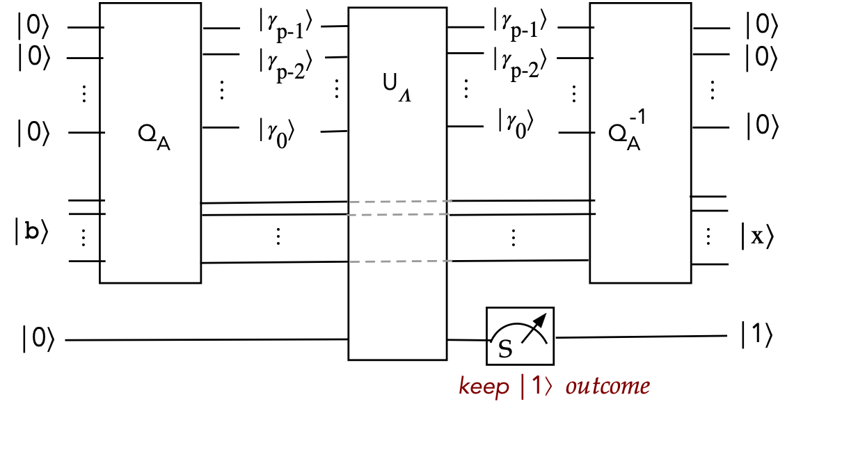
Note:
- We've drawn \(U_\Lambda\) across the middle qubits.
\(\rhd\)
However, \(U_\Lambda\) does not act on them.
- The circuit doesn't show the movement of constants
\(\rhd\)
That's only seen in the algebraic derivation
Finally, let's estimate the time taken.
- The \(Q_A\) unitary is the Quantum Phase Estimation (QPE) algorithm
from Module 12
- We'll assume the unitary \(U = e^{iA}\) can be implemented
efficiently.
- Since QPE needs control-\(U\), we'll assume that can be
implemented efficiently as well.
- The QPE circuit requires control-\(U\) to be applied \(2^p\) times.
- Thus, \(p\) would need to be reasonably small.
- The inverse-QFT is polynomial in \(p\): \(O(p^2)\).
- \(U_\Lambda\) has \(2^p\) different combinations of controls
- Each requires \(p-1\) additional qubits in sequence (successive
\(\cnot\)'s)
- This implies \(O(2^p p)\) gates across.
Lastly, we'll next examine a useful technique as an alternative
way to compute \(U_\Lambda\)
In-Class Exercise 4:
Consider a rotation by \(\alpha\) with \(p=1\) and where the control
for activating the rotation is \(\kt{c_1c_2} = \kt{10}\). Derive
the 3-qubit unitary for this case. [Hint: use projectors]
13.7
Building block: binary digit-based additive rotations
We'll first flesh out a generally useful building block:
- Let
$$
\theta \eql 0.\theta_{p-1}\theta_{p-2}\ldots\theta_{0}
$$
be a \(p\) binary-digit number and
$$
\alpha \eql 2\pi\left( 0.\theta_{p-1}\theta_{p-2}\ldots\theta_{0} \right)
$$
be an angle constructed from \(\theta\)'s digits
- We will design the following circuit:
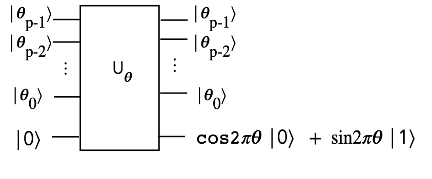
- Then, later, we will pick \(\theta\) such that
$$
\sin 2\pi\theta \eql \frac{c}{\lambda}
$$
to apply this circuit to HHL.
- Let's look at a \(p=3\) example to explain:
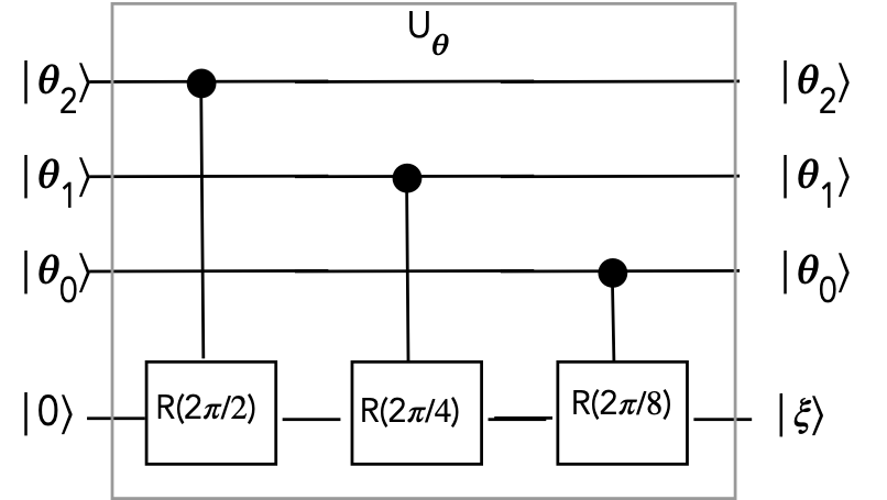
- Suppose, for example, \(0.\theta_{2}\theta_{1}\theta_{0} = 0.011\)
- Then, only the latter two rotations are activated
- This results in
$$\eqb{
\kt{\xi} & \eql &
R\left(\frac{2\pi}{8}\right) \: R\left(\frac{2\pi}{4}\right) \: \kt{0} \\
& \eql &
R\left(\frac{2\pi}{8} + \frac{2\pi}{4} \right) \: \kt{0} \\
& \eql &
R\left(0\cdot \frac{2\pi}{2} + 1\cdot\frac{2\pi}{4} + 1\cdot\frac{2\pi}{8} \right) \: \kt{0} \\
& \eql &
R\left( 2\pi(0\cdot 2^{-1} + 1\cdot 2^{-2} + 1\cdot 2^{-3} )\right) \: \kt{0}\\
& \eql &
R\left( 2\pi(0.011)\right) \: \kt{0}\\
& \eql &
R\left( 2\pi(0.\theta_{2}\theta_{1}\theta_{0})\right) \: \kt{0}\\
& \eql &
\sin\left( 2\pi(0.\theta_{2}\theta_{1}\theta_{0})\right) \: \kt{0}
\; + \;
\cos\left( 2\pi(0.\theta_{2}\theta_{1}\theta_{0})\right) \: \kt{1}\\
& \approx &
\sin\left( 2\pi\theta\right) \: \kt{0}
\; + \;
\cos\left( 2\pi\theta\right) \: \kt{1}\\
}$$
- Note the addition of angles when rotations are applied in
sequence
- The selection of which rotations is achieved by the bits
\(\theta_{2}\theta_{1}\theta_{0}\)
- In general, for \(p\) digits (\(p\) control qubits), we'll need
\(p\) controlled rotations.
- All that's needed now is to use this to produce \(\frac{c}{\lambda}\)
for HHL.
13.8
Approach #2: HHL via additive rotations
What we will do is build \(U_\Lambda\) in a different way:
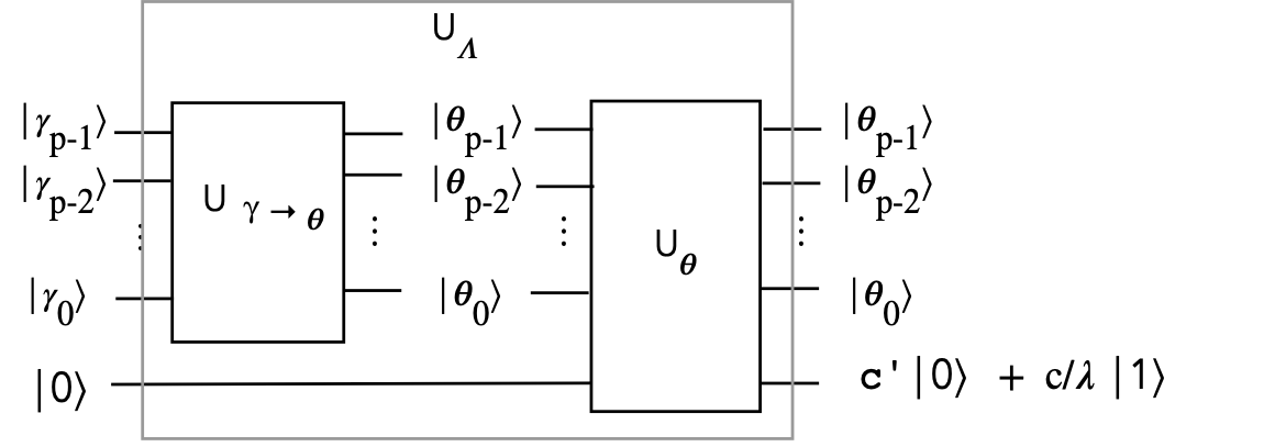
- The previous section showed how to construct \(U_\theta\).
\(\rhd\)
What remains: how to construct \(U_{\gamma\to\theta}\)
- Earlier, we saw how to achieve the mapping from the digits
\(\gamma_{p-1}\gamma_{p-2}\ldots\gamma_0\)
to \(\frac{c}{\lambda}\)
- To see which \(\theta\) digits produce the same:
- Focus on the \(\kt{1}\) part of the last qubit
- The last-qubit output of \(U_\theta\) is
$$
\sin\left( 2\pi\theta\right) \: \kt{0}
\; + \;
\cos\left( 2\pi\theta\right) \: \kt{1}
$$
- Set
$$
\cos\left( 2\pi\theta\right) \eql \frac{c}{\lambda}
$$
to get the \(\theta\) digits for any particular \(\lambda\)
- For a particular \(\lambda\):
- We already know which \(\gamma\) digits produce this \(\lambda\)
- The above analysis shows which \(\theta\) digits produce this \(\lambda\)
- Thus, the \(U_{\gamma\to\theta}\) circuit needs to map
\(\gamma\) digits to \(\theta\) digits
(for each possible \(\lambda\))
- Clearly, this amounts to mapping binary-digit patterns of
\(\gamma\) digits to \(\theta\) digits
\(\rhd\)
A permutation mapping of standard-basis vectors
- This permutation mapping (a \(2^p \times 2^p\) matrix) can be designed
once and for all, and optimized.
- The same mapping can be used for any matrix \(A\).
- So, now we have a slightly more efficient implementation of
\(U_\Lambda\):
- One single \(2^p \times 2^p\) unitary to use across all \(A\)'s
- \(p\) singly-controlled rotations in \(U_\theta\)
- The rest of the HHL implementation uses QPE as before.
Summary
What have we learned in this module?
- The HHL algorithm aims to solve the classical problem \({\bf Ax} = {\bf b}\)
- We note that solving such systems is a building block in
many computations, including in machine learning (such as regression).
- There are many assumptions in the HHL algorithm that make it
impractical to use for a single case.
- More likely, if \(\kt{b}\) is already present from other quantum
calculations, then HHL can produce an approximate \(\kt{x}\) quickly.
- Perhaps most usefully:
- HHL involves many building blocks useful in general
- It introduces the idea of adjusting amplitudes
of eigenvectors, without explicitly knowing the eigenvectors
- How to construct constants and move them about
- HHL is a good starting point for understanding how quantum
algorithms can apply to machine learning.
- What remains: setting up the \(\kt{b}\) vector
(Or, for that matter, any multi-qubit state)
\(\rhd\)
Next module
References
The material in this module is summarized from various sources:
- Aaronson, S. Read the fine print. Nature Phys 11, 291–293 (2015).
- Berry, D.W., Childs, A.M. and Kothari, R (2015).
Hamiltonian simulation with nearly optimal dependence on all parameters.
IEEE FOCS.
- Cao, Y., Daskin, A., Frankel, S., and Kais, S. (2012). Quantum circuit design for solving linear systems of equations. Molecular Physics, 110(15–16), 1675–1680.
- Dervovic, D., Herbster, M., Mountney, P., Severini, S., Usher, N., and Wossnig, L. (2018). Quantum linear systems algorithms: a primer. ArXiv, abs/1802.08227.
- Harrow, A.W., Hassidim, A., and Lloyd, S (2009).
Quantum Algorithm for Linear Systems of Equations.
Phys. Rev. Lett. 103, 150502.
- Shewchuk, J.R (1994). An Introduction to the Conjugate Gradient Method Without the Agonizing Pain. Technical Report. Carnegie Mellon University.
- Zaman, A., Morrell, H. and Wong, H (2023). A Step-by-Step HHL Algorithm Walkthrough to Enhance Understanding of Critical Quantum Computing Concepts. IEEE Access, Vol. 11, pp.77117-77131.